
Introduction to Numerical Analysis: Polynomial Interpolation
Introduction to Polynomial Interpolation
Polynomial interpolation is the procedure of fitting a polynomial of degree  to a set of
  data points. For example, if we have two data points, then we can fit a polynomial of degree 1 (i.e., a linear function) between the two points. If we have three data points, then we can fit a polynomial of the second degree (a parabola) that passes through the three points. Figure 1 shows fitting polynomials of degrees 1, 2, 3, and 4, to sets of 2, 3, 4, and 5 data points. The polynomial equation for each curve is shown in the title for each graph.
Polynomial interpolation relies on the fact that for every data points, there is a unique polynomial of degree that passes through these data points. This fact relies on the Fundamental Theorem of Algebra that states that every degree polynomial has exactly roots. So, if two degree polynomials  and
and  agree on points, then, their difference
  is a polynomial of degree but has roots which implies that
  .
.
To find the unique polynomial of degree that passes through data points, we need to solve a linear set of equations with the coefficients of the polynomial being the unknowns. Let  be the
  data point where
  . Then, we have:
![\[ \begin{split} a_0+a_1x_1+a_2x_1^2+\cdots +a_nx_1^n&=y_1\\ a_0+a_1x_2+a_2x_2^2+\cdots +a_nx_2^n&=y_2\\ &\vdots \\ a_0+a_1x_{n+1}+a_2x_{n+1}^2+\cdots +a_nx_{n+1}^n&=y_{n+1} \end{split} \]](https://engcourses-uofa.ca/wp-content/ql-cache/quicklatex.com-a4ee44770453f85fa43c69307aa79aed_l3.png "Rendered by QuickLaTeX.com")
Which can be written as follows in matrix form:
(1) 
The above system can be solved to find the values of the coefficients  which would ensure that the polynomial curve
  passes through the data points.
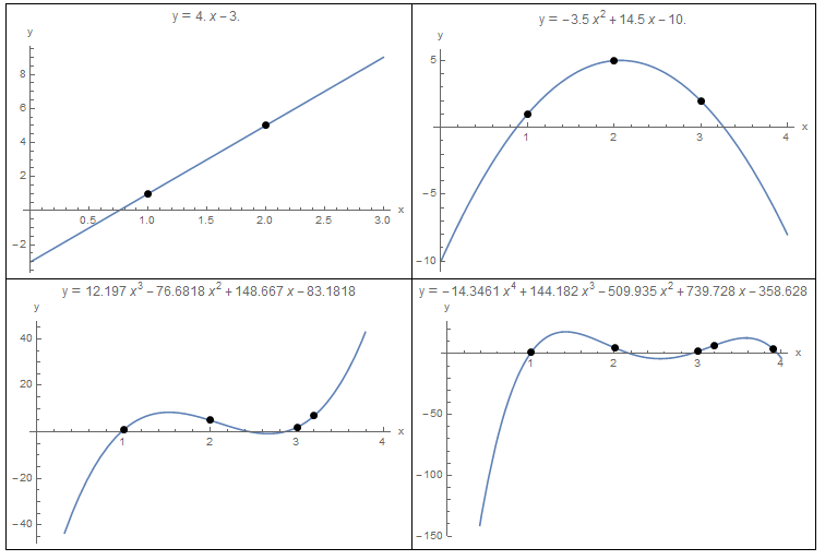
Figure 1. Polynomial Interpolation for 2, 3, 4, and 5 data points.
Data = {{1, 1}, {2, 5.}};
y = InterpolatingPolynomial[Data, x];
a = Plot[y, {x, 0, 3}, Epilog -> {PointSize[Large], Point[Data]}, AxesLabel -> {"x", "y"}, ImageSize -> Medium, PlotLabel -> "y" == Expand[y]];

Data = {{1, 1}, {2, 5.}, {3, 2}};
y = InterpolatingPolynomial[Data, x];
b = Plot[y, {x, 0, 4}, Epilog -> {PointSize[Large], Point[Data]},AxesLabel -> {"x", "y"}, ImageSize -> Medium, PlotLabel -> "y" == Expand[y]];

Data = {{1, 1}, {2, 5}, {3, 2}, {3.2, 7}};
y = InterpolatingPolynomial[Data, x];
c = Plot[y, {x, 0, 4}, Epilog -> {PointSize[Large], Point[Data]}, AxesLabel -> {"x", "y"}, ImageSize -> Medium, PlotLabel -> "y" == Expand[y]];

Data = {{1, 1}, {2, 5}, {3, 2}, {3.2, 7}, {3.9, 4}};
y = InterpolatingPolynomial[Data, x];
d = Plot[y, {x, 0, 4}, Epilog -> {PointSize[Large], Point[Data]}, AxesLabel -> {"x", "y"}, ImageSize -> Medium, PlotLabel -> "y" == Expand[y]];
Grid[{{a, b}, {c, d}}, Frame -> All]
Example
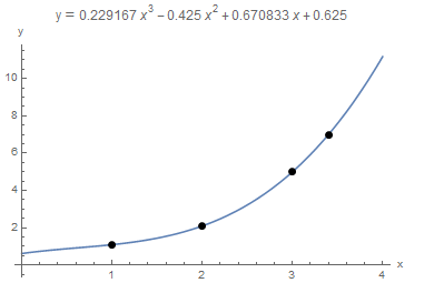
Find an interpolating polynomial that would fit the data points  .
.
Solution
There are four data points, so, we can fit a third degree polynomial whose coefficients can be found by solving the following system of four linear equations:
![\[ \left(\begin{matrix}1&1&1&1\\1&2&2^2&2^3\\1&3&3^2&3^3\\ 1&3.4&3.4^2&3.4^3 \end{matrix}\right)\left(\begin{array}{c}a_0\\a_1\\a_2\\a_3\end{array}\right)=\left(\begin{array}{c}1.1\\2.1\\5\\7\end{array}\right) \]](https://engcourses-uofa.ca/wp-content/ql-cache/quicklatex.com-319209d76ec32a55165850383d5c0ae6_l3.png "Rendered by QuickLaTeX.com")
Solving the above system yields:
![\[ a_0=0.625\qquad a_1=0.670833\qquad a_2=-0.425 \qquad a_3=0.229167 \]](https://engcourses-uofa.ca/wp-content/ql-cache/quicklatex.com-f23b7ccad53985e5d041a4bb674b609d_l3.png "Rendered by QuickLaTeX.com")
Therefore, the interpolating polynomial that would pass through all four data points is:
![\[ y=0.625+0.670833x-0.425x^2+0.229167x^3 \]](https://engcourses-uofa.ca/wp-content/ql-cache/quicklatex.com-98a2434b3f8b1bcb25038b14602651bb_l3.png "Rendered by QuickLaTeX.com")
The following Mathematica code was used to solve the above equations and produce the plot below:
View Mathematica Code
M = {{1, 1, 1, 1}, {1, 2, 4, 2^3}, {1, 3, 9, 27}, {1, 3.4, 3.4^2, 3.4^3}};
yv = {1.1, 2.1, 5, 7}
a = Inverse[M].yv
y = a[[1]] + a[[2]]*x + a[[3]]*x^2 + a[[4]]*x^3
Plot[y, {x, 0, 4}, Epilog -> {PointSize[Large],  Point[{{1, 1.1}, {2, 2.1}, {3, 5}, {3.4, 7}}]}, AxesLabel -> {"x", "y"}, ImageSize -> Medium, PlotLabel -> "y" == Expand[y]]
Mathematica also has a built-in “InterpolatingPolynomial[Data,x]” function that would automatically form and solve the above equation as shown below. Simply provide the data points as a list and Mathematica would produce the interpolating polynomial as a function of “x”.
View Mathematica Code
Data = {{1, 1.1}, {2, 2.1}, {3, 5}, {3.4, 7}};
y = InterpolatingPolynomial[Data, x];
Plot[y, {x, 0, 4}, Epilog -> {PointSize[Large], Point[Data]}, AxesLabel -> {"x", "y"}, ImageSize -> Medium, PlotLabel -> "y" == Expand[y]]
Disadvantages
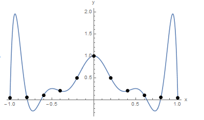
There are various disadvantages to this interpolating polynomials method. The first disadvantage is that as the number of data points gets bigger, the linear systems of equations that need to be solved become ill-conditioned. In other words, the matrix that needs to be converted would be composed of both small and very large numbers, a situation which is prone to round-off errors. Another major disadvantage is that as the number of data points increases, the order of the interpolating polynomial increases as well. By construction, the polynomial would pass through the data points. However, for large order ( ), the polynomial would be oscillating wildly between the data points leading to large errors in the interpolated values. The following example illustrates this:
Example
Consider the following 11 data points: (-1.00,0.038),(-0.80,0.058),(-0.60,0.100),(-0.4,0.200),(-0.20,0.500),(0.00,1.000),(0.20,0.500),(0.40,0.200),(0.60,0.100),(0.80,0.0580),(1.00,0.038). Using the InterpolatingPolynomial function in Mathematica the 10th order polynomial that would fit through all these points has the form:
![\[ y=1-16.8551x^2+123.356x^4-381.407x^6+494.843x^8-220.9x^{10} \]](https://engcourses-uofa.ca/wp-content/ql-cache/quicklatex.com-7f74507662b25eb818f3a481058220eb_l3.png "Rendered by QuickLaTeX.com")
From the plot below, the polynomial indeed passes through the 11 points, however, in between the points it oscillates wildly. In fact, for  the values of the polynomial are much higher than the values at the points
  and
and  which were used for the interpolation:
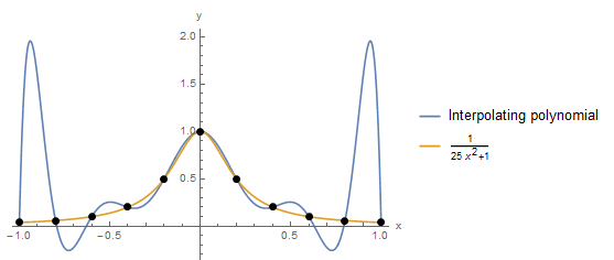
It is worth noting that the data points were actually generated using the Runge function:
![\[ y=\frac{1}{1+25x^2} \]](https://engcourses-uofa.ca/wp-content/ql-cache/quicklatex.com-0b808b41f4f17c760533b7605cdb2c20_l3.png "Rendered by QuickLaTeX.com")
When  is plotted versus the interpolation function, it is clear that the polynomial interpolation function, if used instead of would produce erroneous results for values outside of the control points. In fact, Runge used this example in the nineteenth century to show that using higher order polynomials to approximate functions does not always improve accuracy but can have detrimental effects on the values of the function in the intervals between the control points.
Data = {{-1, 0.038}, {-0.8, 0.058}, {-0.60, 0.10}, {-0.4, 0.20}, {-0.2, 0.50}, {0, 1}, {0.2, 0.5}, {0.4, 0.2}, {0.6, 0.1}, {0.8, 0.058}, {1, 0.038}};
y = InterpolatingPolynomial[Data, x]
Chop[Expand[y]]
Plot[y, {x, -1, 1}, Epilog -> {PointSize[Large], Point[Data]}, AxesLabel -> {"x", "y"}, ImageSize -> Medium]
y2 = 1/(1 + 25 x^2)
Plot[{y, y2}, {x, -1, 1}, Epilog -> {PointSize[Large], Point[Data]}, AxesLabel -> {"x", "y"}, ImageSize -> Medium, PlotLegends -> {"Interpolating polynomial", y2}]
Newton Interpolating Polynomials
As stated above, the matrix formed in Equation 1 can be ill-conditioned and difficult to find an inverse for. A simpler method can be used to find the interpolating polynomial using Newton’s Interpolating Polynomials formula for fitting a polynomial of degree through data points with  :
:
![\[ f_n(x)=b_1+b_2(x-x_1)+b_3(x-x_1)(x-x_2)+\cdots+b_{n+1}(x-x_1)(x-x_2)\cdots(x-x_n) \]](https://engcourses-uofa.ca/wp-content/ql-cache/quicklatex.com-68440c188f4ed3e251f5a1c7d4bd02ae_l3.png "Rendered by QuickLaTeX.com")
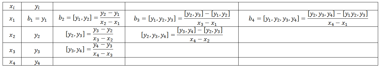
where the coefficients  are defined recursively using the divided differences as follows:
![\[\begin{split} b_1&=y_1\\ b_2&=[y_1,y_2]=\frac{y_2-y_1}{x_2-x_1}\\ b_3&=[y_1,y_2,y_3]=\frac{[y_2,y_3]-[y_1,y_2]}{x_3-x_1}=\frac{\frac{y_3-y_2}{x_3-x_2}-\frac{y_2-y_1}{x_2-x_1}}{x_3-x_1}\\ \vdots &\\ b_{n+1}&=[y_1,y_2,y_3,\cdots,y_{n+1}]=\frac{[y_2,y_3,\cdots,y_{n+1}]-[y_1,y_2,y_3,\cdots,y_{n}]}{x_{n+1}-x_1} \end{split} \]](https://engcourses-uofa.ca/wp-content/ql-cache/quicklatex.com-49413b6651e0e40147b1cf17f2d55841_l3.png "Rendered by QuickLaTeX.com")
This recursive divided differences are illustrated in the following table:
The following Mathematica code implements a recursive function “f” that produces the coefficients .
View Mathematica Code
Data = {{1, 3}, {4, 5}, {5, 6}, {6, 8}, {7, 8}};
f[anydata_] := If[Length[anydata] == 1, anydata[[1, 2]], If[Length[anydata] ==2, (anydata[[2, 2]] - anydata[[1, 2]])/(anydata[[2, 1]] -anydata[[1, 1]]), (f[Drop[anydata, 1]] - f[Drop[anydata, -1]])/(anydata[[Length[anydata], 1]] - anydata[[1, 1]])]]
NP[anydata_] := Sum[f[anydata[[1 ;; i]]]*Product[(x - anydata[[j, 1]]), {j, 1, i - 1}], {i, 1, Length[anydata]}]
(*Using the Newton polynomial function*)
y = Expand[NP[Data]]
(*Using the interpolating polynomial built-in function*)
y2 = Expand[InterpolatingPolynomial[Data, x]]
Newton’s formula for generating an interpolating polynomial adopts a form similar to that of a Taylor’s polynomial but is based on finite differences rather than the derivatives. I.e., the coefficients are calculated using finite difference. One advantage to this form is that the degree of a Newton’s interpolating polynomial can be increased (or decreased) automatically by adding (or removing) more terms corresponding to new points without discarding existing terms.
Example
Using Newton’s interpolating polynomials, find the interpolating polynomial to the data: (1,1),(2,5).
Solution
We have two data points, so, we will create a polynomial of the first degree. Therefore:
![\[ b_1=y_1=1\qquad b_2=\frac{5-1}{2-1}=4 \]](https://engcourses-uofa.ca/wp-content/ql-cache/quicklatex.com-46b71e9109599c501be0012c0c1ea7a7_l3.png "Rendered by QuickLaTeX.com")
Therefore, the interpolating polynomial has the form:
![\[ y=1+4(x-1)=1+4x-4=-3+4x \]](https://engcourses-uofa.ca/wp-content/ql-cache/quicklatex.com-389fcac9e9f9eb5a3f52731463060a27_l3.png "Rendered by QuickLaTeX.com")
Example
Using Newton’s interpolating polynomials, find the interpolating polynomial to the data: (1,1),(2,5),(3,2).
Solution
We have three data points, so, we will create a polynomial of the second degree. Therefore:
![\[ b_1=y_1=1\qquad b_2=\frac{5-1}{2-1}=4 \qquad b_3=\frac{\frac{2-5}{3-2}-\frac{5-1}{2-1}}{3-1}=-3.5 \]](https://engcourses-uofa.ca/wp-content/ql-cache/quicklatex.com-6f8535cbef6d0207e01fd453bc945a3c_l3.png "Rendered by QuickLaTeX.com")
Therefore, the interpolating polynomial has the form:
![\[ y=1+4(x-1)-3.5(x-1)(x-2)=-3.5x^2+14.5x-10 \]](https://engcourses-uofa.ca/wp-content/ql-cache/quicklatex.com-aa0844431a26b7ca2b649ed2d1f1ce57_l3.png "Rendered by QuickLaTeX.com")
Example
Using Newton’s interpolating polynomials, find the interpolating polynomial to the data: (1,1),(2,5),(3,2),(3.2,7),(3.9,4).
Solution
The divided difference table for these data points were created in excel as follows:
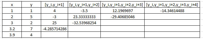
Therefore, the Newton’s Interpolating Polynomial has the form:
![\[\begin{split} y=&1+4(x-1)-3.5(x-1)(x-2)+12.19697(x-1)(x-2)(x-3)\\ &-14.346144(x-1)(x-2)(x-3)(x-3.2)\\ =&-14.3461x^4+144.181x^3-509.935x^2+739.728x-358.628 \end{split} \]](https://engcourses-uofa.ca/wp-content/ql-cache/quicklatex.com-4a31ba4a94d14fac179a9dfcecc645c1_l3.png "Rendered by QuickLaTeX.com")
Lagrange Interpolating Polynomials
Another equivalent method to find the interpolating polynomials is using the Lagrange Polynomials. Given data points:  , then the Lagrange polynomial of degree that fits through the data points has the form:
![\[ f_n(x)=L_1y_1+L_2y_2+L_3y_3+\cdots+L_{n+1}y_{n+1}=\sum_{i=1}^{n+1}L_iy_i \]](https://engcourses-uofa.ca/wp-content/ql-cache/quicklatex.com-834283952a8430f969796efd1c3d4f6a_l3.png "Rendered by QuickLaTeX.com")
where
![\[ L_i=\prod_{j=1,j\neq i}^{n+1}\frac{x-x_j}{x_i-x_j} \]](https://engcourses-uofa.ca/wp-content/ql-cache/quicklatex.com-fdea4e0984a88748fcb446425406f729_l3.png "Rendered by QuickLaTeX.com")
In the following Mathematica code a Lagrange polynomial procedure is created to output the Lagrange polynomials.
View Mathematica CodeData = {{1, 3}, {4, 5}, {5, 6}, {6, 8}, {7, 8}};
Lagrange[anydata_] := Sum[anydata[[i, 2]]*LP[anydata, i], {i, 1, Length[anydata]}]
LP[anydata_, i_] := (newdata = Drop[anydata, {i}]; Product[(x - newdata[[j, 1]])/(anydata[[i, 1]] - newdata[[j, 1]]), {j, 1, Length[newdata]}])
(*Using the Lagrange polynomial function*)
y = Expand[Lagrange[Data]]
(*Using the interpolating polynomial built-in function*)
y2 = Expand[InterpolatingPolynomial[Data, x]]
The Lagrange interpolating polynomials produce the same polynomial as the general method and the Newton’s interpolating polynomials. The examples used for the Newton’s interpolating polynomials will be repeated here.
Example
Using Lagrange interpolating polynomials, find the interpolating polynomial to the data: (1,1),(2,5).
Solution
We have two data points, so, we will create a polynomial of the first degree. Therefore, the interpolating polynomial has the form:
![\[\begin{split} y&=L_1y_1+L_2y_2=\left(\frac{x-x_2}{x_1-x_2}\right)y_1+\left(\frac{x-x_1}{x_2-x_1}\right)y_2\\ &=\left(\frac{x-2}{1-2}\right)\times 1+\left(\frac{x-1}{2-1}\right)\times 5\\ &=4x-3 \end{split} \]](https://engcourses-uofa.ca/wp-content/ql-cache/quicklatex.com-42aa52be6aec9303aebcd4f875765139_l3.png "Rendered by QuickLaTeX.com")
Example
Using Lagrange interpolating polynomials, find the interpolating polynomial to the data: (1,1),(2,5),(3,2).
Solution
We have three data points, so, we will create a polynomial of the second degree. Using Lagrange polynomials:
![\[\begin{split} y&=L_1y_1+L_2y_2+L_3y_3\\ &=\frac{(x-x_2)(x-x_3)}{(x_1-x_2)(x_1-x_3)}y_1+\frac{(x-x_1)(x-x_3)}{(x_2-x_1)(x_2-x_3)}y_2+\frac{(x-x_1)(x-x_2)}{(x_3-x_1)(x_3-x_2)}y_3\\ &=\frac{(x-2)(x-3)}{(1-2)(1-3)}(1)+\frac{(x-1)(x-3)}{(2-1)(2-3)}(5)+\frac{(x-1)(x-2)}{(3-1)(3-2)}(2)\\ &=-3.5x^2+14.5x-10 \end{split} \]](https://engcourses-uofa.ca/wp-content/ql-cache/quicklatex.com-dcfb410585446daf2f95fd2028ac0638_l3.png "Rendered by QuickLaTeX.com")
Example
Using Lagrange polynomials, find the interpolating polynomial to the data: (1,1),(2,5),(3,2),(3.2,7),(3.9,4).
Solution
A fourth order polynomial would be needed to pass through five data points. Using Lagrange polynomials, the required function has the form:
![\[\begin{split} y=&\frac{(x-x_2)(x-x_3)(x-x_4)(x-x_5)}{(x_1-x_2)(x_1-x_3)(x_1-x_4)(x_1-x_5)}y_1+\frac{(x-x_1)(x-x_3)(x-x_4)(x-x_5)}{(x_2-x_1)(x_2-x_3)(x_2-x_4)(x_2-x_5)}y_2\\ &+\frac{(x-x_1)(x-x_2)(x-x_4)(x-x_5)}{(x_3-x_1)(x_3-x_2)(x_3-x_4)(x_3-x_5)}y_3+\frac{(x-x_1)(x-x_2)(x-x_3)(x-x_5)}{(x_4-x_1)(x_4-x_2)(x_4-x_3)(x_4-x_5)}y_4\\ &+\frac{(x-x_1)(x-x_2)(x-x_3)(x-x_4)}{(x_5-x_1)(x_5-x_2)(x_5-x_3)(x_5-x_4)}y_5\\ =&-14.3461x^4+144.181x^3-509.935x^2+739.728x-358.628 \end{split} \]](https://engcourses-uofa.ca/wp-content/ql-cache/quicklatex.com-9e01d63ce3b6e26d4cea4d2e26c3f281_l3.png "Rendered by QuickLaTeX.com")
Extrapolation
Extrapolation is the process of predicting a value that lies outside the range of the known base points. Extrapolation using polynomials should be treated with extreme care. For example, the Runge function described above predicts, when  , the value of
  . Had we used extrapolation using the fitted polynomial, the predicted value would have been
  which does not really follow the trend of the interpolated points!
Problems
- Derive the Newton interpolating polynomial and the Lagrange polynomial formulas.
- Find 5 examples where an engineer could have some discrete experimental observations for specific instances of a variable
 and would be seeking a relationship to describe versus .
 - The following data points provide the distance in m on a plate and the corresponding measured temperature in Celsius (0,80), (2,53.5), (4,38.43), (6,30.39), (8,30). Find an interpolating polynomial that fits through all the data points. Plot the curve showing the interpolating polynomial and mark the data points on the curve. Use the interpolating polynomial to estimate the temperature at
 .
. - Using the same data given in the previous problem, estimate the temperature at using linear, quadratic, third, and fourth order Newton polynomial interpolation. For each case, pick enough points for the order of interpolation. Do you get the same answer? Comment on the results.
- Repeat the previous problem using linear, quadratic, third order, and fourth Lagrange polynomial interpolation. Comment on your answer.
- The following data provides the average tuition fees in Canadian dollars for engineering students in Alberta from 2010 to 2014 (2010,5401),(2012,5886), (2013,5871), (2014,5929). Use an interpolating polynomial to find an estimate for the tuition fees in 2011. (Data source). Compare your result to the actual value reported by Stats Canada which is: 5815 Canadian dollars.
- The concentration of a certain toxin in a system of lakes has been monitored at intervals from 1993 to 2003 and was reported as (1993,120), (1995, 127), (1997, 130), (1999, 152), (2001, 182), (2003,198). Using polynomial interpolation, estimate the concentration in 2002. What happens if you remove the first two data points, do you get the same estimate? Comment on your answer.