Engineering at Alberta Courses » Newton Raphson Method

Open Methods: Newton Raphson Method

The Method

The Newton-Raphson method is one of the most used methods of all root-finding methods. The reason for its success is that it converges very fast in most cases. In addition, it can be extended quite easily to multi-variable equations. To find the root of the equation $f(x_t)=0$ , the Newton-Raphson method depends on the Taylor Series Expansion of the function around the estimate $x_i$ to find a better estimate $x_{i+1}$ :

$f(x_{i+1})=f(x_i)+f'(x_i)(x_{i+1}-x_i)+\mathcal O (h^2)$

where $x_{i+1}$ is the estimate of the root after iteration $i+1$ and $x_i$ is the estimate at iteration $i$ . Assuming $f(x_{i+1})=0$ and rearranging:

$x_{i+1}\approx x_i-\frac{f(x_i)}{f'(x_i)}$

The procedure is as follows. Setting an initial guess $x_0$ , tolerance $\varepsilon_s$ , and maximum number of iterations $N$ :
At iteration $i$ , calculate $x_i\approx x_{i-1}-\frac{f(x_{i-1})}{f'(x_{i-1})}$ and $\varepsilon_r$ . If $\varepsilon_r\leq \varepsilon_s$ or if $i\geq N$ , stop the procedure. Otherwise repeat.
Note: unlike the previous methods, the Newton-Raphson method relies on calculating the first derivative of the function $f(x)$ . This makes the procedure very fast, however, it has two disadvantages. The first is that this procedure doesn’t work if the function $f(x)$ is not differentiable. Second, the inverse $(f'(x_{i}))^{-1}$ can be slow to calculate when dealing with multi-variable equations.

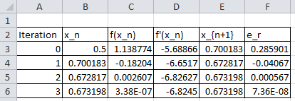
Example

As an example, let’s consider the function $f(x)=\sin{5x}+\cos{2x}$ . The derivative of $f$ is $f'(x)=5\cos{5x}-2\sin{2x}$ . Setting the maximum number of iterations $N=100$ , $\varepsilon_s=0.0005$ , $x_0=0.5$ , the following is the Microsoft Excel table produced:
NR1

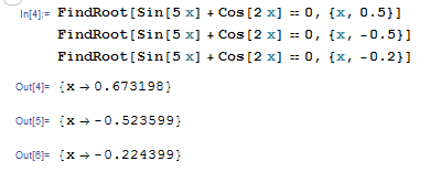
Mathematica has a built-in algorithm for the Newton-Raphson method. The function “FindRoot[lhs==rhs,{x,x0}]” applies the Newton-Raphson method with the initial guess being “x0”. The following is a screenshot of the input and output of the built-in function evaluating the roots based on three initial guesses.
NR2

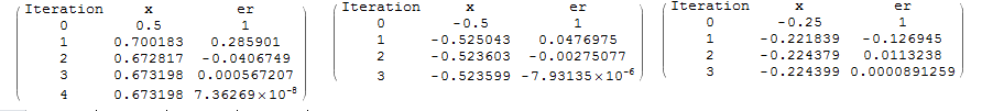
Alternatively, a Mathematica code can be written to implement the Newton-Raphson method with the following output for three different initial guesses:
NR3

View Mathematica Code

Clear[x]
f[x_] := Sin[5 x] + Cos[2 x]
fp = D[f[x], x]
xtable = {-0.25};
er = {1};
es = 0.0005;
MaxIter = 100;
i = 1;
While[And[i <= MaxIter, Abs[er[[i]]] > es], xnew = xtable[[i]] - (f[xtable[[i]]]/fp /. x -> xtable[[i]]);  xtable = Append[xtable, xnew]; ernew = (xnew - xtable[[i]])/xnew;  er = Append[er, ernew]; i++];
T = Length[xtable];
SolutionTable = Table[{i - 1, xtable[[i]], er[[i]]}, {i, 1, T}];
SolutionTable1 = {"Iteration", "x", "er"};
T = Prepend[SolutionTable, SolutionTable1];
T // MatrixForm

View Python Code

import sympy as sp
import pandas as pd

def f(x): return sp.sin(5*x) + sp.cos(2*x)
x = sp.symbols('x')
fp = f(x).diff(x)
xtable = [-0.25]
er = [1]
es = 0.0005
MaxIter = 100
i = 0
while i <= MaxIter and abs(er[i]) > es:
  xnew = xtable[i] - (f(xtable[i])/fp.subs(x,xtable[i]))
  xtable.append(xnew)
  ernew = (xnew - xtable[i])/xnew
  er.append(ernew)
  i+=1
SolutionTable = [[i, xtable[i], er[i]] for i in range(len(xtable))];
sol = pd.DataFrame(SolutionTable,columns=["Iteration", "x", "er"])
display(sol)

# Scipy's root function
import numpy as np
from scipy.optimize import root
def f(x):
  return np.sin(5*x) + np.cos(2*x)
sol = root(f,[0])
print("Scipy's Root: ",sol.x)

The following MATLAB code runs the Newton-Raphson method to find the root of a function $f(x)$ with derivative $f'(x)$ and initial guess $x_0$ . The value of the estimate and approximate relative error at each iteration is displayed in the command window. Additionally, two plots are produced to visualize how the iterations and the errors progress. You need to pass the function f(x) and its derivative df(x) to the newton-raphson method along with the initial guess as newtonraphson(@(x) f(x), @(x) df(x), x0). For example, try newtonraphson(@(x) sin(5.*x)+cos(2.*x), @(x) 5.*cos(5.*x)-2.*sin(2.*x),0.4)

MATLAB file Download

Analysis of Convergence of the Newton-Raphson Method

The error in the Newton-Raphson Method can be roughly estimated as follows. The estimate $x_{i+1}$ is related to the previous estimate $x_i$ using the equation:

$x_{i+1}=x_i-\frac{f(x_i)}{f'(x_i)}\Rightarrow 0=f(x_i)+f'(x_i)(x_{i+1}-x_i)$

Additionally, using Taylor’s theorem, and if $x_t$ is the true root with $f(x_t)=0$ we have:

$f(x_t)=0=f(x_i)+f'(x_i)(x_t-x_i)+\frac{f''(\xi)}{2!}{(x_t-x_i)^2}$

for some $\xi$ in the interval between $x_i$ and $x_t$ . Subtracting the above two equations yields:

$0=f'(x_i)(x_t-x_{i+1})+\frac{f''(\xi)}{2!}{(x_t-x_i)^2}$

Since $E_{i+1}=x_t-x_{i+1}$ and $E_i=x_t-x_i$ then:

(1) $\begin{equation*} E_{i+1}=-\frac{f''(\xi)}{2!f'(x_i)}{E_i^2} \end{equation*}$

If the method is converging, we have $f''(\xi)\approx f''(x_t)$ and $f'(\xi)\approx f'(x_t)$ therefore:

$E_{i+1}\propto E_i^2$

Therefore, the error is squared after each iteration, i.e., the number of correct decimal places approximately doubles with each iteration. This behaviour is called quadratic convergence. Look at the tables in the Newton-Raphson example above and compare the relative error after each step!

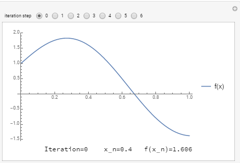
The following tool can be used to visualize how the Newton-Raphson method works. Using the slope $f'(x_i)$ , the difference $x_{i+1}-x_i$ can be calculated and thus, the value of the new estimate $x_{i+1}$ can be computed accordingly. Use the slider to see how fast the method converges to the true solution using $\varepsilon_s=0.0005$ , $x_0=0.4$ , and solving for the root of $f(x)=\sin[5x]+\cos[2x]=0$ .

View Mathematica code

Manipulate[
 f[x_] := Sin[5 x] + Cos[2 x];
 fp = D[f[x], x];
 xtable = {0.4};
 er = {1};
 es = 0.0005;
 MaxIter = 100;
 i = 1;
 While[And[i <= MaxIter, Abs[er[[i]]] > es], xnew = xtable[[i]] - (f[xtable[[i]]]/fp /. x -> xtable[[i]]); xtable = Append[xtable, xnew]; ernew = (xnew - xtable[[i]])/xnew; er = Append[er, ernew]; i++];
 T = Length[xtable];
 SolutionTable = Table[{i - 1, xtable[[i]], er[[i]]}, {i, 1, T}];
 SolutionTable1 = {"Iteration", "x", "er"};
 T = Prepend[SolutionTable, SolutionTable1];
  LineTable1 = Table[{{T[[i, 2]], 0}, {T[[i, 2]], f[T[[i, 2]]]}, {T[[i + 1, 2]],0}}, {i, 2, n - 1}];
 Grid[{{Plot[f[x], {x, 0, 1}, PlotLegends -> {"f(x)"}, ImageSize -> Medium,  Epilog -> {Dashed, Line[LineTable1]}]}, {Row[{"Iteration=", n - 2, "    x_n=", T[[n, 2]], "   f(x_n)=", f[T[[n, 2]]]}]}}], {n, 2, 7, 1}]

View Python Code

import numpy as np
import sympy as sp
import matplotlib.pyplot as plt
from ipywidgets.widgets import interact

def f(x): return sp.sin(5*x) + sp.cos(2*x)
x = sp.symbols('x')
fp = f(x).diff(x)

@interact(n=(2,7,1))
def update(n=2):
  xtable = [0.4]
  er = [1]
  es = 0.0005
  MaxIter = 100
  i = 0
  while i <= MaxIter and abs(er[i]) > es:
    xnew = xtable[i] - (f(xtable[i])/fp.subs(x,xtable[i]))
    xtable.append(xnew)
    ernew = (xnew - xtable[i])/xnew
    er.append(ernew)
    i+=1
  SolutionTable = [[i - 1, xtable[i], er[i]] for i in range(len(xtable))]
  LineTable = [[],[]]
  for i in range(n-2):
    LineTable[0].extend([SolutionTable[i][1], SolutionTable[i][1], SolutionTable[i + 1][1]])
    LineTable[1].extend([0, f(SolutionTable[i][1]), 0])
  
  x_val = np.arange(0,1.1,0.03)
  y_val = np.sin(5*x_val) + np.cos(2*x_val)
  plt.plot(x_val,y_val, label="f(x)")
  plt.plot(LineTable[0],LineTable[1],'k--')
  plt.legend(); plt.grid(); plt.show()
  print("Iteration =",n-2," x_n =",round(SolutionTable[n-2][1],5)," f(x_n) =",f(SolutionTable[n-2][1]))

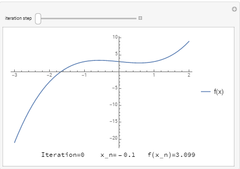
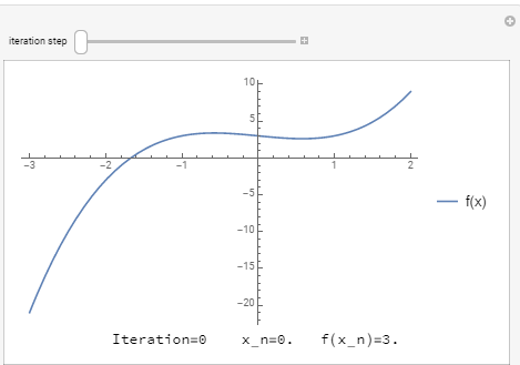
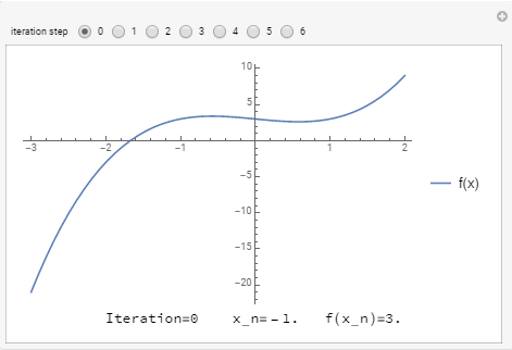
Depending on the shape of the function and the initial guess, the Newton-Raphson method can get stuck around the locations of oscillations of the function. The tool below visualizes the algorithm when trying to find the root of $f(x)=x^3-x+3=0$ with an initial guess of $x_0=-0.1$ . It takes 33 iterations before reaching convergence.

Depending on the shape of the function and the initial guess, the Newton-Raphson method can get stuck in a loop. The tool below visualizes the algorithm when trying to find the root of $f(x)=x^3-x+3=0$ with an initial guess of $x_0=0$ . The algorithm goes into an infinite loop.

In general, an initial guess that is close enough to the true root will guarantee quick convergence. The tool below visualizes the algorithm when trying to find the root of $f(x)=x^3-x+3=0$ with an initial guess of $x_0=-1$ . The algorithm quickly converges to the desired root.

The following is the Mathematica code used to generate one of the tools above:

View Mathematica Code

Manipulate[
 f[x_] := x^3 - x + 3;
 fp = D[f[x], x];
 xtable = {-0.1};
 er = {1.};
 es = 0.0005;
 MaxIter = 100;
 i = 1;
 While[And[i <= MaxIter, Abs[er[[i]]] > es], xnew = xtable[[i]] - (f[xtable[[i]]]/fp /. x -> xtable[[i]]); xtable = Append[xtable, xnew]; ernew = (xnew - xtable[[i]])/xnew; er = Append[er, ernew]; i++];
 T = Length[xtable];
 SolutionTable = Table[{i - 1, xtable[[i]], er[[i]]}, {i, 1, T}];
 SolutionTable1 = {"Iteration", "x", "er"};
 T = Prepend[SolutionTable, SolutionTable1]; 
 LineTable1 =   Table[{{T[[i, 2]], 0}, {T[[i, 2]], f[T[[i, 2]]]}, {T[[i + 1, 2]], 0}}, {i, 2, n - 1}];
 Grid[{{Plot[f[x], {x, -3, 2}, PlotLegends -> {"f(x)"}, ImageSize -> Medium, Epilog -> {Dashed, Line[LineTable1]}]}, {Row[{"Iteration=", n - 2, "    x_n=", T[[n, 2]], "   f(x_n)=", f[T[[n, 2]]]}]}}] , {n, 2, 33, 1}]

View Python Code

import numpy as np
import sympy as sp
import matplotlib.pyplot as plt
from ipywidgets.widgets import interact

def f(x): return x**3 - x + 3
x = sp.symbols('x')
fp = f(x).diff(x)

@interact(n=(2,33,1))
def update(n=2):
  xtable = [-0.1]
  er = [1]
  es = 0.0005
  MaxIter = 100
  i = 0
  while i <= MaxIter and abs(er[i]) > es:
    xnew = xtable[i] - (f(xtable[i])/fp.subs(x,xtable[i]))
    xtable.append(xnew)
    ernew = (xnew - xtable[i])/xnew
    er.append(ernew)
    i+=1
  SolutionTable = [[i - 1, xtable[i], er[i]] for i in range(len(xtable))]
  LineTable = [[],[]]
  for i in range(n-2):
    LineTable[0].extend([SolutionTable[i][1], SolutionTable[i][1], SolutionTable[i + 1][1]])
    LineTable[1].extend([0, f(SolutionTable[i][1]), 0])
  
  x_val = np.arange(-3,2.2,0.03)
  y_val = x_val**3 - x_val + 3
  plt.plot(x_val,y_val, label="f(x)")
  plt.plot(LineTable[0],LineTable[1],'k--')
  plt.xlim(-3,2.2); plt.ylim(-25,10)
  plt.legend(); plt.grid(); plt.show()
  print("Iteration =",n-2," x_n =",round(SolutionTable[n-2][1],5)," f(x_n) =",round(f(SolutionTable[n-2][1]),5))

Lecture video

Page Comments

Lei Zhang says:

January 29, 2021 at 9:40 pm

In the Microsoft Excel table, the # of iteration should be 1,2,3,4, not 0,1,2,3.

Reply
1. Samer Adeeb says:
  
  January 29, 2021 at 9:43 pm
  
  Either choice is fine
  
  Reply
mary says:

April 29, 2023 at 11:05 am

I have the newtenRaphson method in matlab but I have faced a problem or waring message.
please could you help me?

Reply

Open Educational Resources

Open Methods: Newton Raphson Method

The Method

Example

Analysis of Convergence of the Newton-Raphson Method

Lecture video

Page Comments

Leave a Reply to mary Cancel reply