Solution Methods for IVPs: Heun’s Method

Heun’s Method

Heun’s method provides a slight modification to both the implicit and explicit Euler methods. Consider the following IVP:

Assuming that the value of the dependent variable (say ) is known at an initial value , then, we have:

If the trapezoidal rule is used for the right-hand side with one interval we obtain:

where the error term is inherited from the use of the trapezoidal integration rule. Therefore an estimate for is given by:

Using this estimate, the local truncation error is thus proportional to the cube of the step size. If the errors from each interval are added together, with being the number of intervals and the total length , then, the total error is:

which is better than both the implicit and explicit Euler methods. Note that Heun’s method is essentially a slight modification to the Euler’s method in which the slope used to calculate the value of at the next time point is used as the average slope at and at . Heun’s method can be implemented in two ways. One way is to use the slope at to calculate an initial estimate . Then, the estimate for would be calculated based on the slopes at and . Alternatively, the Newton-Raphson method or the fixed-point iteration method can be used to solve directly for . We will only adopt the first way. The following Mathematica code presents a procedure to utilize Heun’s method. The procedure is essentially similar to the ones presented in the Euler methods except for the step to calculate the new estimate .

HeunMethod[fp_, x0_, h_, t0_, tmax_] := 
(n = (tmax - t0)/h + 1;
  xtable = Table[0, {i, 1, n}];
  xtable[[1]] = x0;
  Do[xi0 = xtable[[i - 1]] + h*fp[xtable[[i - 1]], t0 + (i - 2) h]; 
   xtable[[i]] = xtable[[i - 1]] + h (fp[xtable[[i - 1]], t0 + (i - 2) h] +fp[xi0, t0 + (i - 1) h])/2, {i, 2, n}];
  Data = Table[{t0 + (i - 1)*h, xtable[[i]]}, {i, 1, n}];
  Data)

def HeunMethod(fp, x0, h, t0, tmax):
  n = int((tmax - t0)/h + 1)
  xtable = [0 for i in range(n)]
  xtable[0] = x0
  for i in range(1,n):
    xi0 = xtable[i - 1] + h*fp(xtable[i - 1], t0 + (i - 1)*h)
    xtable[i] =  xtable[i - 1] + h*(fp(xtable[i - 1], t0 + (i - 1)*h) + fp(xi0, t0 + i*h))/2
  Data = [[t0 + i*h, xtable[i]] for i in range(n)]
  return Data

Example

Solve Example 4 above using Heun’s method.

Solution

Heun’s method is implemented by first assuming an estimate for based on the explicit Euler method:

Then, the estimate for is calculated as:

Setting , , , and , an initial estimate for is given by:

Using this information, the slope at can be calculated and used to estimate :

Similarly, an initial estimate for is given by:

Using this information, the slope at can be calculated and used to estimate :

Proceeding iteratively gives the values of up to . The Microsoft Excel file Heun.xlsx provides the required calculations.

The following graph shows the produced numerical data (black dots) overlapping the exact solution (blue line). The Mathematica code is given below.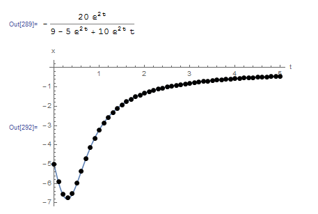

HeunMethod[fp_, x0_, h_, t0_, tmax_] := (n = (tmax - t0)/h + 1;
  xtable = Table[0, {i, 1, n}];
  xtable[[1]] = x0;
  Do[xi0 = xtable[[i - 1]] + h*fp[xtable[[i - 1]], t0 + (i - 2) h]; 
   xtable[[i]] =  xtable[[i - 1]] +   h (fp[xtable[[i - 1]], t0 + (i - 2) h] +  fp[xi0, t0 + (i - 1) h])/2, {i, 2, n}];
  Data = Table[{t0 + (i - 1)*h, xtable[[i]]}, {i, 1, n}];
  Data)
Clear[x, xtable]
a = DSolve[{x'[t] == t*x[t]^2 + 2*x[t], x[0] == -5}, x, t];
x = x[t] /. a[[1]]
fp[x_, t_] := t*x^2 + 2*x;
Data2 = HeunMethod[fp, -5.0, 0.1, 0, 5];
Plot[x, {t, 0, 5}, Epilog -> {PointSize[Large], Point[Data2]}, AxesOrigin -> {0, 0}, AxesLabel -> {"t", "x"}, PlotRange -> All]
Title = {"t_i", "x_i"};
Data2 = Prepend[Data2, Title];
Data2 // MatrixForm

# UPGRADE: need Sympy 1.2 or later, upgrade by running: "!pip install sympy --upgrade" in a code cell
# !pip install sympy --upgrade
import numpy as np
import sympy as sp
import matplotlib.pyplot as plt
sp.init_printing(use_latex=True)

def HeunMethod(fp, x0, h, t0, tmax):
  n = int((tmax - t0)/h + 1)
  xtable = [0 for i in range(n)]
  xtable[0] = x0
  for i in range(1,n):
    xi0 = xtable[i - 1] + h*fp(xtable[i - 1], t0 + (i - 1)*h)
    xtable[i] =  xtable[i - 1] + h*(fp(xtable[i - 1], t0 + (i - 1)*h) + fp(xi0, t0 + i*h))/2
  Data = [[t0 + i*h, xtable[i]] for i in range(n)]
  return Data

x = sp.Function('x')
t = sp.symbols('t')
sol = sp.dsolve(x(t).diff(t) - t*x(t)**2 - 2*x(t), ics={x(0): -5})
display(sol)
def fp(x, t): return t*x**2 + 2*x
Data = HeunMethod(fp, -5.0, 0.1, 0, 5)
x_val = np.arange(0,5,0.01)
plt.plot(x_val, [sol.subs(t, i).rhs for i in x_val])
plt.scatter([point[0] for point in Data],[point[1] for point in Data],c='k')
plt.xlabel("t"); plt.ylabel("x")
plt.grid(); plt.show()
print(["t_i", "x_i"],"\n",np.vstack(Data))

The following tool provides a comparison between the explicit Euler method and Heun’s method. Notice that around , the function varies highly in comparison to the rest of the domain. The biggest difference between Heun’s method and the Euler method can be seen when around this area. Heun’s method is able to trace the curve while the Euler method has higher deviations.

Lecture Video