
Introduction to Numerical Analysis: Numerical Integration
Introduction
Integrals arise naturally in the fields of engineering to describe quantities that are functions of infinitesimal data. For example, if the velocity of a moving object for a particular period of time is known, then the change of position of the moving object can be estimated by summing the velocity at discrete time points multiplied by the corresponding time intervals between the discrete points. The accuracy of the change in position can be increased by decreasing the number of discrete time points, i.e., by reducing the time intervals between the discrete points. The formal definition of an integral of a function ![f:[a,b]\rightarrow \mathbb{R}](https://engcourses-uofa.ca/wp-content/ql-cache/quicklatex.com-602dc0a5221796cd029651364476c9ef_l3.png "Rendered by QuickLaTeX.com") is the signed area of the region under the curve
is the signed area of the region under the curve  between the points
  and
and  . The definite integral is denoted by:
![\[ \int_{a}^b\!f(x)\,\mathrm{d}x \]](https://engcourses-uofa.ca/wp-content/ql-cache/quicklatex.com-1eaa0cc4969bf56c6ec8694f25b249cb_l3.png "Rendered by QuickLaTeX.com")
Fundamental Theorem of Calculus
The fundamental theorem of calculus links the concepts of integration and differentiation; roughly speaking, they are the converse of each other. The fundamental theorem of calculus can be stated as follows:
Part I
Let be continuous, and let ![F:[a,b]\rightarrow \mathbb{R}](https://engcourses-uofa.ca/wp-content/ql-cache/quicklatex.com-8f15d39360fb368268c0a775591abd15_l3.png "Rendered by QuickLaTeX.com") be the function defined such that
be the function defined such that ![\forall x\in[a,b]](https://engcourses-uofa.ca/wp-content/ql-cache/quicklatex.com-ee63298b0bb6f908aa2b79bd957b11dc_l3.png "Rendered by QuickLaTeX.com") :
:
![\[ F(x)=\int_{a}^x\!f(x)\,\mathrm{d}x \]](https://engcourses-uofa.ca/wp-content/ql-cache/quicklatex.com-768f25553f1a02a368b0df83ef73ca99_l3.png "Rendered by QuickLaTeX.com")
then,  is uniformly continuous on
 ![[a,b]](https://engcourses-uofa.ca/wp-content/ql-cache/quicklatex.com-1f90ba537767823131bb8d396cdc5a9c_l3.png "Rendered by QuickLaTeX.com") , is differentiable on
, is differentiable on  , and
, and  is the derivative of (also stated as is the antiderivative of ):
![\[ \frac{\mathrm{d}F}{\mathrm{d}x}=f(x) \]](https://engcourses-uofa.ca/wp-content/ql-cache/quicklatex.com-69d19a34ddb3932b6a56e7c47a565fda_l3.png "Rendered by QuickLaTeX.com")
In other words, the first part asserts that if is continuous on the interval , then, an antiderivative always exists; is the derivative of a function that can be defined as  with
with ![x\in[a,b]](https://engcourses-uofa.ca/wp-content/ql-cache/quicklatex.com-7bdc9e9b79b72dde0a30288760e0fe60_l3.png "Rendered by QuickLaTeX.com") .
.
Part II
Let and be two continuous functions such that  (i.e., is the derivative of , or is an antiderivative of ), then:
![\[ \int_{a}^b\!f(x)\,\mathrm{d}x=F(b)-F(a) \]](https://engcourses-uofa.ca/wp-content/ql-cache/quicklatex.com-30cf2220d4fd7cca07ff335d8214a321_l3.png "Rendered by QuickLaTeX.com")
The second part states that if has an antiderivative , then can be used to calculate the definite integral of on the interval .
For visual proofs of the fundamental theorem of calculus, check out this page.
Numerical Integration
The fundamental theorem of calculus allows the calculation of  using the antiderivative of . However, if the antiderivative is not available, a numerical procedure can be employed to calculate the integral or the area under the curve. Historically, the term “Quadrature” was used to mean calculating areas. For example, the Gauss numerical integration scheme that will be studied later is also called the Gauss quadrature. The basic problem in numerical integration is to calculate an approximate solution to the definite integral of a function
 ![f:[a,b]](https://engcourses-uofa.ca/wp-content/ql-cache/quicklatex.com-f9ef6059ed642d0a774671c54562f008_l3.png "Rendered by QuickLaTeX.com") .
.
Riemann Integral
One of the early definitions of the integral of a function is the limit:
![\[ \int_{a}^b\!f(x)\,\mathrm{d}x=\lim_{\max{\Delta x_k}\rightarrow 0 } \sum_{k=1}^n f(x_k^*)\Delta x_k \]](https://engcourses-uofa.ca/wp-content/ql-cache/quicklatex.com-8db18b970c18cc9df64571a1e4401d76_l3.png "Rendered by QuickLaTeX.com")
where  ,
,  , and
, and  is an arbitrary point such that
 ![x_k^*\in [x_k,x_{k+1}]](https://engcourses-uofa.ca/wp-content/ql-cache/quicklatex.com-1c640bcf7e39a83f233f2cdbba32b682_l3.png "Rendered by QuickLaTeX.com") . If
. If  is the sum of the areas of vertical rectangles arranged next to each other and whose top sides touch the function at arbitrary points, then, the Riemann integral is the limit of this sum as the maximum width of the vertical rectangles approaches zero. A function is “Riemann integrable” if the limit above (the limit of ) exists as the width of the rectangles gets smaller and smaller. In this course, we are always dealing with continuous functions. For continuous functions, the limit always exists and thus, all continuous functions are “Riemann integrable”.
Newton-Cotes Formulas
The Newton-Cotes formulas rely on replacing the function or tabulated data with an interpolating polynomial that is easy to integrate. In this case, the required integral is evaluated as:
![\[ I=\int_{a}^b\!f(x)\,\mathrm{d}x\approx \int_{a}^b\!f_n(x)\,\mathrm{d}x \]](https://engcourses-uofa.ca/wp-content/ql-cache/quicklatex.com-b33de56dc89802c1c270868ac31dde6b_l3.png "Rendered by QuickLaTeX.com")
where  is a polynomial of degree
  which can be constructed to pass through
  data points in the interval .
Example
Consider the function ![f:[0,1]\rightarrow \mathbb{R}](https://engcourses-uofa.ca/wp-content/ql-cache/quicklatex.com-69c326526bfd63b1733489dc8b5bea8c_l3.png "Rendered by QuickLaTeX.com") defined as:
defined as:
![\[ f(x)=2-x^2+0.1\cos{\left(\frac{2\pi x}{0.7}\right)} \]](https://engcourses-uofa.ca/wp-content/ql-cache/quicklatex.com-913f1ce9868603f80b795274307b02ff_l3.png "Rendered by QuickLaTeX.com")
Calculate the exact integral:
![\[ I=\int_{0}^1\!f(x)\,\mathrm{d}x \]](https://engcourses-uofa.ca/wp-content/ql-cache/quicklatex.com-b7ffa6f0bf865fef8fd2e50dafa73f17_l3.png "Rendered by QuickLaTeX.com")
Using steps sizes of  , fit an interpolating polynomial to the values of the function at the generated points and calculate the integral by integrating the polynomial. Compare the exact with the interpolating polynomial.
Solution
The exact integral can be calculated using Mathematica to be:
![\[ I=\int_{0}^1\!f(x)\,\mathrm{d}x=1.6715 \]](https://engcourses-uofa.ca/wp-content/ql-cache/quicklatex.com-fc0647691816582df66c2237aa2efe01_l3.png "Rendered by QuickLaTeX.com")
The following figures show the interpolating polynomial fitted through data points at step sizes of 0.1, 0.2, 0.5, and 1. The exact integral compared with the numerical integration scheme evaluated by integrating the interpolating polynomial is shown under each curve. Naturally, the higher the degree of the polynomial, the closer the numerical value to the exact value.
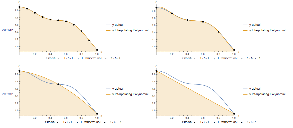
The resulting interpolating polynomials are given by:
![\[\begin{split} y_{h=0.1}&=2.1 + 0.0161419 x - 5.48942 x^2 + 5.32445 x^3 - 6.11881 x^4 + 123.581 x^5 - 356.658 x^6\\ & + 389.096 x^7 - 159.091 x^8 - 6.69727 x^9 + 14.8471 x^{10}\\ y_{h=0.2}&=2.1 + 1.11382 x - 18.0584 x^2 + 53.5143 x^3 - 61.493 x^4 + 23.7332 x^5\\ y_{h=0.5}&=2.1 - 0.298911 x - 0.891185 x^2\\ y_{h=1}&=2.1-1.1901x \end{split} \]](https://engcourses-uofa.ca/wp-content/ql-cache/quicklatex.com-b2c9c1040e265ab0dcb883951a55b5b7_l3.png "Rendered by QuickLaTeX.com")
Integrating the above formulas is straightforward and the resulting values are:
![\[\begin{split} I_{h=0.1}&=1.6715\\ I_{h=0.2}&=1.67294\\ I_{h=0.5}&=1.65348\\ I_{h=1}&=1.50495 \end{split} \]](https://engcourses-uofa.ca/wp-content/ql-cache/quicklatex.com-525cf037ac2d1595c744a1ba1ae7771d_l3.png "Rendered by QuickLaTeX.com")
The following is the Mathematica code used.
View Mathematica Code
h = {0.1, 0.2, 0.5, 1};
n = Table[1/h[[i]] + 1, {i, 1, 4}];
y = 2 - x^2 + 0.1*Cos[2 Pi*x/0.7];
Data = Table[{h[[i]]*(j - 1), (y /. x -> h[[i]]*(j - 1.0))}, {i, 1, 4}, {j, 1, n[[i]]}];
Data // MatrixForm;
p = Table[InterpolatingPolynomial[Data[[i]], x], {i, 1, 4}];
a1 = Plot[{y, p[[1]]}, {x, 0, 1},   Epilog -> {PointSize[Large], Point[Data[[1]]]},   AxesLabel -> {"x", "y"}, BaseStyle -> Bold, ImageSize -> Medium,   PlotRange -> All, Filling -> {2 -> Axis},   PlotLegends -> {"y actual", "y Interpolating Polynomial"}];
a2 = Plot[{y, p[[2]]}, {x, 0, 1},    Epilog -> {PointSize[Large], Point[Data[[2]]]},    AxesLabel -> {"x", "y"}, BaseStyle -> Bold, ImageSize -> Medium,    PlotRange -> All, Filling -> {2 -> Axis},    PlotLegends -> {"y actual", "y Interpolating Polynomial"}];
a3 = Plot[{y, p[[3]]}, {x, 0, 1},    Epilog -> {PointSize[Large], Point[Data[[3]]]},    AxesLabel -> {"x", "y"}, BaseStyle -> Bold, ImageSize -> Medium,    PlotRange -> All, Filling -> {2 -> Axis},    PlotLegends -> {"y actual", "y Interpolating Polynomial"}];
a4 = Plot[{y, p[[4]]}, {x, 0, 1},    Epilog -> {PointSize[Large], Point[Data[[4]]]},    AxesLabel -> {"x", "y"}, BaseStyle -> Bold, ImageSize -> Medium,    PlotRange -> All, Filling -> {2 -> Axis},    PlotLegends -> {"y actual", "y Interpolating Polynomial"}];
Iexact = Integrate[y, {x, 0, 1}];
Inumerical = Table[Integrate[p[[i]], {x, 0, 1}], {i, 1, 4}];
atext = Table[Grid[{{"I exact = ", Iexact, ", I numerical = ", Inumerical[[i]]}}], {i, 1, 4}];
Grid[{{a1, a2}, {atext[[1]], atext[[2]]}}]
Grid[{{a3, a4}, {atext[[3]], atext[[4]]}}]
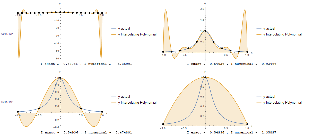
However, as described in the interpolating polynomial section, the larger the degree of the polynomial, the more susceptible it is to oscillations. As an example, the previous problem is repeated with the Runge function defined on the interval from -1 to 1. The figure below shows that using many points leads to large oscillations in the interpolating polynomial which renders the numerical integration largely inaccurate. When fewer points are used, the interpolating polynomial is still highly inaccurate. Therefore, the Newton-Cotes formulas can be applied by simply subdividing the interval into smaller subintervals and applying the Newton-Cotes formulas to each subinterval and adding the results. This process is called: “Composite rules”. The rectangle method, trapezoidal rule, and Simpson’s rules presented in the following sections are specific examples of the composite Newton-Cotes formulas.
h = {0.1, 0.2, 0.5, 1};
n = Table[2/h[[i]] + 1, {i, 1, 4}];
y = 1.0/(1 + 25 x^2);
Data = Table[{-1 +    h[[i]]*(j - 1), (y /. x -> -1 + h[[i]]*(j - 1.0))}, {i, 1,     4}, {j, 1, n[[i]]}];
Data // MatrixForm;
p = Table[InterpolatingPolynomial[Data[[i]], x], {i, 1, 4}];
a1 = Plot[{y, p[[1]]}, {x, -1, 1},    Epilog -> {PointSize[Large], Point[Data[[1]]]},    AxesLabel -> {"x", "y"}, BaseStyle -> Bold, ImageSize -> Medium,    PlotRange -> All, Filling -> {2 -> Axis},    PlotLegends -> {"y actual", "y Interpolating Polynomial"}];
a2 = Plot[{y, p[[2]]}, {x, -1, 1},    Epilog -> {PointSize[Large], Point[Data[[2]]]},    AxesLabel -> {"x", "y"}, BaseStyle -> Bold, ImageSize -> Medium,    PlotRange -> All, Filling -> {2 -> Axis},    PlotLegends -> {"y actual", "y Interpolating Polynomial"}];
a3 = Plot[{y, p[[3]]}, {x, -1, 1},    Epilog -> {PointSize[Large], Point[Data[[3]]]},    AxesLabel -> {"x", "y"}, BaseStyle -> Bold, ImageSize -> Medium,    PlotRange -> All, Filling -> {2 -> Axis},    PlotLegends -> {"y actual", "y Interpolating Polynomial"}];
a4 = Plot[{y, p[[4]]}, {x, -1, 1},    Epilog -> {PointSize[Large], Point[Data[[4]]]},    AxesLabel -> {"x", "y"}, BaseStyle -> Bold, ImageSize -> Medium,    PlotRange -> All, Filling -> {2 -> Axis},    PlotLegends -> {"y actual", "y Interpolating Polynomial"}];
Iexact = Integrate[y, {x, -1, 1}];
Inumerical = Table[Integrate[p[[i]], {x, -1, 1}], {i, 1, 4}];

atext = Table[   Grid[{{"I exact = ", Iexact, ", I numerical = ",  Inumerical[[i]]}}], {i, 1, 4}];
Grid[{{a1, a2}, {atext[[1]], atext[[2]]}}]
Grid[{{a3, a4}, {atext[[3]], atext[[4]]}}]
Rectangle Method
Let . The rectangle method utilizes the Riemann integral definition to calculate an approximate estimate for the area under the curve by drawing many rectangles with very small width adjacent to each other between the graph of the function and the  axis. For simplicity, the width of the rectangles is chosen to be constant. Let be the number of intervals with
  and constant spacing
  . The rectangle method can be implemented in one of the following three ways:
![\[\begin{split} I_1&=\int_{a}^b\!f(x)\,\mathrm{d}x\approx h\sum_{i=1}^{n}f(x_{i-1})\\ I_2&=\int_{a}^b\!f(x)\,\mathrm{d}x\approx h\sum_{i=1}^{n}f\left(\frac{x_{i-1}+x_{i}}{2}\right)\\ I_3&=\int_{a}^b\!f(x)\,\mathrm{d}x\approx h\sum_{i=1}^{n}f(x_{i}) \end{split} \]](https://engcourses-uofa.ca/wp-content/ql-cache/quicklatex.com-40b546d84c498d8430b9daeafa0b6479_l3.png "Rendered by QuickLaTeX.com")
If  and
and  are the left and right points defining the rectangle number
  , then
  assumes that the height of the rectangle is equal to
  ,
,  assumes that the height of the rectangle is equal to
  , and
, and  assumes that the height of the rectangle is equal to
  . is called the midpoint rule.
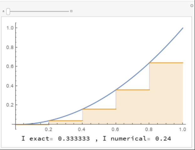
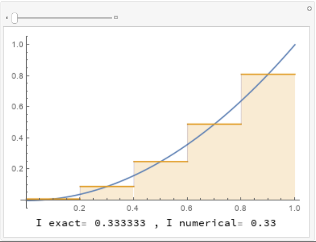
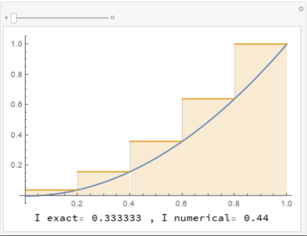
To illustrate the difference, consider the function  on the interval
 ![[0,1]](https://engcourses-uofa.ca/wp-content/ql-cache/quicklatex.com-a8b36d8d3c0436b5a9c763cbff76f47a_l3.png "Rendered by QuickLaTeX.com") . The exact integral can be calculated as
. The exact integral can be calculated as
![\[ I_{\mbox{exact}}=\frac{x^3}{3}\bigg|_{x=0}^{x=1}=0.3333 \]](https://engcourses-uofa.ca/wp-content/ql-cache/quicklatex.com-b5ce16cd32c4956c652a512a09c4b6da_l3.png "Rendered by QuickLaTeX.com")
The following three tools show the implementation of the rectangle method for numerically integrating the function using , , and , respectively. For , each rectangle touches the graph of the function at the top left corner of the rectangle. For , each rectangle touches the graph of the function at the mid point of the top side. For , each rectangle touches the graph of the function at the top right corner of the rectangle. The areas of the rectangles are calculated underneath each curve. Use the slider to increase the number of rectangles to see how many rectangles are needed to get a good approximation for the area under the curve.
The following Mathematica code can be used to numerically integrate any function on the interval using the three options for the rectangle method.
View Mathematica Code
I1[f_, a_, b_, n_] := (h = (b - a)/n; Sum[f[a + (i - 1)*h]*h, {i, 1, n}])
I2[f_, a_, b_, n_] := (h = (b - a)/n; Sum[f[a + (i - 1/2)*h]*h, {i, 1, n}])
I3[f_, a_, b_, n_] := (h = (b - a)/n; Sum[f[a + (i)*h]*h, {i, 1, n}])
f[x_] := x^2;
I1[f, 0, 1, 13.0]
I2[f, 0, 1, 13.0]
I3[f, 0, 1, 13.0]
Error Analysis
Taylor’s theorem can be used to find how the error changes as the step size  decreases. First, let’s consider (the same applies to ). The error in the calculation of rectangle number between the points and will be estimated. Using Taylor’s theorem,
 ![\forall x\in[x_{i-1},x_{i}], \exists \xi\in[x_{i-1},x]](https://engcourses-uofa.ca/wp-content/ql-cache/quicklatex.com-fe93a07818df72a11422b1855cdcdef9_l3.png "Rendered by QuickLaTeX.com") such that:
such that:
![\[ f(x)=f(x_{i-1})+f'(\xi)(x-x_{i-1}) \]](https://engcourses-uofa.ca/wp-content/ql-cache/quicklatex.com-9a8eb366d03b972408630df77b4068fa_l3.png "Rendered by QuickLaTeX.com")
The error in the integral using this rectangle can be calculated as follows:
![\[\begin{split} |E_i|&=\left|\int_{x_{i-1}}^{x_{i}}\!f(x)-f(x_{i-1})\,\mathrm{d}x\right|=\left|\int_{x_{i-1}}^{x_{i}}\!f'(\xi)(x-x_{i-1})\,\mathrm{d}x\right|\\ &\leq \max_{\xi\in[x_{i-1},x_i]}|f'(\xi)|\frac{(x-x_{i-1})^2}{2}\bigg|_{x_{i-1}}^{x_i}=\max_{\xi\in[x_{i-1},x_i]}|f'(\xi)|\frac{h^2}{2} \end{split} \]](https://engcourses-uofa.ca/wp-content/ql-cache/quicklatex.com-a59cd86aa604ae772523f56ea70e7003_l3.png "Rendered by QuickLaTeX.com")
If is the number of subdivisions (number of rectangles), i.e.,  , then:
![\[ |E|=|nE_i| \leq \max_{\xi\in[a,b]}|f'(\xi)| n\frac{h^2}{2}=\max_{\xi\in[a,b]}|f'(\xi)| (b-a)\frac{h}{2} \]](https://engcourses-uofa.ca/wp-content/ql-cache/quicklatex.com-dc3a53b2fde998b18179b46c5f6b491c_l3.png "Rendered by QuickLaTeX.com")
In other words, the total error is bounded by a term that is directly proportional to . When decreases, the error bound decreases proportionally. Of course when goes to zero, the error goes to zero as well.
(Midpoint rule) provides a faster convergence rate, or a more accurate approximation as the error is bounded by a term that is directly proportional to  as will be shown here.
Using Taylor’s theorem, such that:
![\[ f(x)=f(x_{m})+f'(x_i)(x-x_{m})+f''(\xi)\frac{(x-x_{m})}{2} \]](https://engcourses-uofa.ca/wp-content/ql-cache/quicklatex.com-ea8bda5829ee5f360032eb7a14515f0f_l3.png "Rendered by QuickLaTeX.com")
Where  . The error in the integral using this rectangle can be calculated as follows:
![\[\begin{split} |E_i|&=\left|\int_{x_{i-1}}^{x_{i}}\!f(x)-f(x_m)\,\mathrm{d}x\right|=\left|f'(x_i)\int_{x_{i-1}}^{x_{i}}\!(x-x_m)\,\mathrm{d}x+\int_{x_{i-1}}^{x_{i}}\!\frac{f''(\xi)}{2}(x-x_m)^2\,\mathrm{d}x\right|\\ &=\left|f'(x_i)\frac{(x_i-x_m)^2-(x_{i-1}-x_m)^2}{2}+\int_{x_{i-1}}^{x_{i}}\!\frac{f''(\xi)}{2}(x-x_m)^2\,\mathrm{d}x\right|\\ &=\left|0+\int_{x_{i-1}}^{x_{i}}\!\frac{f''(\xi)}{2}(x-x_m)^2\,\mathrm{d}x\right|\\ &\leq \max_{\xi\in[x_{i-1},x_i]}\frac{|f''(\xi)|}{2}\frac{\left(\frac{h}{2}\right)^3-\left(\frac{-h}{2}\right)^3}{3}\\ &\leq \max_{\xi\in[x_{i-1},x_i]}\frac{|f''(\xi)|}{24}h^3 \end{split} \]](https://engcourses-uofa.ca/wp-content/ql-cache/quicklatex.com-62df554ea818ffe9acbd648cfd4505bf_l3.png "Rendered by QuickLaTeX.com")
If is the number of subdivisions (number of rectangles), i.e., , then:
![\[ |E|=|nE_i| \leq \max_{\xi\in[a,b]}|f''(\xi)| n\frac{h^3}{24}=\max_{\xi\in[a,b]}|f''(\xi)| (b-a)\frac{h^2}{24} \]](https://engcourses-uofa.ca/wp-content/ql-cache/quicklatex.com-107774d48c8df30e7525cae831088883_l3.png "Rendered by QuickLaTeX.com")
In other words, the total error is bounded by a term that is directly proportional to which provides faster convergence than . The tools shown above can provide a good illustration of this. With only five rectangles, already provides a very good estimate for the integral compared to both , and .
Example
Using the rectangle method with  , calculate , , and and compare with the exact integral of the function
  on the interval
 ![[0,2]](https://engcourses-uofa.ca/wp-content/ql-cache/quicklatex.com-9ec15e699e72ba501abfc77baca9b5a6_l3.png "Rendered by QuickLaTeX.com") . Then, find the values of required so that the total error obtained by and that obtained by are bounded by 0.001.
. Then, find the values of required so that the total error obtained by and that obtained by are bounded by 0.001.
Solution
Since the spacing can be calculated as:
![\[ h=\frac{b-a}{n}=\frac{2-0}{4}=0.5 \]](https://engcourses-uofa.ca/wp-content/ql-cache/quicklatex.com-2c8da9ed6d782c84319b89a288f8e812_l3.png "Rendered by QuickLaTeX.com")
Therefore,  ,
,  ,
,  ,
,  , and
, and  . The values of the function at these points are given by:
![\[ f(x_0)=e^0=1.00\qquad f(x_1)=e^{0.5}=1.6487 \qquad f(x_2)=e^{1}=2.7183 \]](https://engcourses-uofa.ca/wp-content/ql-cache/quicklatex.com-33ed9ba8fe24b17e0c34898d62bd67a5_l3.png "Rendered by QuickLaTeX.com")
![\[ f(x_3)=e^{1.5}=4.4817 \qquad f(x_4)=e^{2}=7.3891 \]](https://engcourses-uofa.ca/wp-content/ql-cache/quicklatex.com-610e0a3cf46c5151f07a0155272c540e_l3.png "Rendered by QuickLaTeX.com")
According to the rectangle method we have:
![\[\begin{split} I_1&=\sum_{i=1}^{n}f(x_{i-1})h=0.5 (1 + 1.6487 + 2.7183 + 4.4817) = 4.924\\ I_3&=\sum_{i=1}^{n}f(x_{i})h=0.5 (1.6487 + 2.7183 + 4.4817+7.3891) = 8.119 \end{split} \]](https://engcourses-uofa.ca/wp-content/ql-cache/quicklatex.com-2c2e0e978e2bacb0abdc0d0177d14a05_l3.png "Rendered by QuickLaTeX.com")
For , we need to calculate the values of the function at the midpoint of each rectangle:
![\[ f\left(\frac{x_0+x_1}{2}\right)=e^{0.25}=1.284 \qquad f\left(\frac{x_1+x_2}{2}\right)=e^{0.75}=2.117 \]](https://engcourses-uofa.ca/wp-content/ql-cache/quicklatex.com-4d56c020436bf646aa2470f6bee87492_l3.png "Rendered by QuickLaTeX.com")
![\[ f\left(\frac{x_2+x_3}{2}\right)=e^{1.25}=3.49 \qquad f\left(\frac{x_3+x_4}{2}\right)=e^{1.75}=5.755 \]](https://engcourses-uofa.ca/wp-content/ql-cache/quicklatex.com-72bf3ffdf2ed06122b02985b24dea9a4_l3.png "Rendered by QuickLaTeX.com")
Therefore:
![\[ I_2=\sum_{i=1}^{n}f\left(\frac{x_{i-1}+x_{i}}{2}\right)h=0.5(1.284+2.117+3.49+5.755)=6.323 \]](https://engcourses-uofa.ca/wp-content/ql-cache/quicklatex.com-d62a8a1941856edf74343d61af9cbe6e_l3.png "Rendered by QuickLaTeX.com")
The exact integral is given by:
![\[ I=\int_{0}^2\!e^x\,\mathrm{d}x=e^2-e^0=6.38906 \]](https://engcourses-uofa.ca/wp-content/ql-cache/quicklatex.com-bd1e917bfda6d31b7c410c1eea23a606_l3.png "Rendered by QuickLaTeX.com")
Obviously, provides a good approximation with only 4 rectangles!
Error Bounds
The total errors obtained when  are indeed less than the error bounds obtained by the formulas listed above. For and , the error in the estimation is bounded by:
![\[ |E|\leq \max_{\xi\in[a,b]}|f'(\xi)| (b-a)\frac{h}{2}=e^{2}(2-0)\frac{0.5}{2}=3.695 \]](https://engcourses-uofa.ca/wp-content/ql-cache/quicklatex.com-723ea4b51f450af14f87c2a0588159e9_l3.png "Rendered by QuickLaTeX.com")
The errors  and
and  are indeed less than that upper bound. The same formula can be used to find the value of so that the error is bounded by 0.001:
![\[ e^{2}(2-0)\frac{h}{2}=0.001\Rightarrow h=0.000135 \]](https://engcourses-uofa.ca/wp-content/ql-cache/quicklatex.com-f99b54ec92f2e2c0786602a6701a67f0_l3.png "Rendered by QuickLaTeX.com")
Therefore, to guarantee an error less than 0.001 using , the interval will have to be divided into:  rectangles! In this case
  and
and 
Similarly, when the error in the estimate using is bounded by:
![\[ |E|=\max_{\xi\in[a,b]}|f''(\xi)| (b-a)\frac{h^2}{24}=e^2(2-0)\frac{0.5^2}{24}=0.1539 \]](https://engcourses-uofa.ca/wp-content/ql-cache/quicklatex.com-7ef56dacf68a9d987796459ef73b8fc7_l3.png "Rendered by QuickLaTeX.com")
The error  is indeed bounded by that upper error. The same formula can be used to find the value of so that the error is bounded by 0.001:
![\[ e^2(2-0)\frac{h^2}{24}=0.001\Rightarrow h = 0.04 \]](https://engcourses-uofa.ca/wp-content/ql-cache/quicklatex.com-6a70ae0939b364663267311e9fa32df5_l3.png "Rendered by QuickLaTeX.com")
Therefore, to guarantee an error less than 0.001 using , the interval will have to be divided into:  rectangles! In this case
  and
and 
Trapezoidal Rule
Let . By dividing the interval into many subintervals, the trapezoidal rule approximates the area under the curve by linearly interpolating between the values of the function at the junctions of the subintervals, and thus, on each subinterval, the area to be calculated has a shape of a trapezoid. For simplicity, the width of the trapezoids is chosen to be constant. Let be the number of intervals with and constant spacing . The trapezoidal method can be implemented as follows:
![\[ I_T=\int_{a}^b\!f(x)\,\mathrm{d}x\approx \frac{h}{2}\sum_{i=1}^{n}\left(f(x_{i-1})+f(x_i)\right)=\frac{h}{2}(f(x_0)+2f(x_1)+2f(x_2)+\cdots+2f(x_{n-1})+f(x_n)) \]](https://engcourses-uofa.ca/wp-content/ql-cache/quicklatex.com-b325e69659ec7b3bd46ac1838a46ace2_l3.png "Rendered by QuickLaTeX.com")
The following tool illustrates the implementation of the trapezoidal rule for integrating the function ![f:[0,1.5]\rightarrow \mathbb{R}](https://engcourses-uofa.ca/wp-content/ql-cache/quicklatex.com-ec8c4de17311939e21dd2feb6df1c644_l3.png "Rendered by QuickLaTeX.com") defined as:
defined as:
![\[ f(x)= 2 + 2 x + x^2 + \sin{(2 \pi x)} + \cos{(2 \pi \frac{x}{0.5})} \]](https://engcourses-uofa.ca/wp-content/ql-cache/quicklatex.com-06ef319c3f9d81b137d86b12afd52cd0_l3.png "Rendered by QuickLaTeX.com")
Use the slider to see the effect of increasing the number of intervals on the approximation.
The following Mathematica code can be used to numerically integrate any function on the interval using the trapezoidal rule.
View Mathematica Code
IT[f_, a_, b_, n_] := (h = (b - a)/n; Sum[(f[a + (i - 1)*h] + f[a + i*h])*h/2, {i, 1, n}])
f[x_] := 2 + 2 x + x^2 + Sin[2 Pi*x] + Cos[2 Pi*x/0.5];
IT[f, 0, 1.5, 1.0]
IT[f, 0, 1.5, 18.0]
Error Analysis
An extension of Taylor’s theorem can be used to find how the error changes as the step size decreases. Given a function and its interpolating polynomial of degree ( ), the error term between the interpolating polynomial and the function is given by (See this article for a proof):
![\[ f(x)=p_n(x)+\frac{f^{n+1}(\xi)}{(n+1)!}\prod_{i=1}^{n+1}(x-x_{i}) \]](https://engcourses-uofa.ca/wp-content/ql-cache/quicklatex.com-6b9b24a2e69e78f9faa93e4a52b7b64e_l3.png "Rendered by QuickLaTeX.com")
Where  is in the domain of the function and is dependent on the point . The error in the calculation of trapezoidal number between the points and will be estimated based on the above formula assuming a linear interpolation between the points and
  . Therefore:
![\[\begin{split} |E_i|&=\left|\int_{x_{i-1}}^{x_i}\! f(x)-p_1(x)\,\mathrm{d}x\right|=\left|\int_{x_{i-1}}^{x_i}\!\frac{f''(\xi)}{2}(x-x_{i-1})(x-x_i)\,\mathrm{d}x\right|\\ &\leq \max_{\xi\in[x_{i-1},x_i]}\frac{|f''(\xi)|h^3}{12} \end{split} \]](https://engcourses-uofa.ca/wp-content/ql-cache/quicklatex.com-daea4ab11443895affee342f6305bca0_l3.png "Rendered by QuickLaTeX.com")
If is the number of subdivisions (number of trapezoids), i.e., , then:
![\[ |E|=|nE_i|\leq \max_{\xi\in[a,b]}\frac{|f''(\xi)|nh^3}{12}=\max_{\xi\in[a,b]}\frac{|f''(\xi)|(b-a)h^2}{12} \]](https://engcourses-uofa.ca/wp-content/ql-cache/quicklatex.com-e079b8ed89fd04e7ed2560d3ca7855a8_l3.png "Rendered by QuickLaTeX.com")
Example
Using the trapezoidal rule with , calculate  and compare with the exact integral of the function on the interval . Find the value of so that the error is less than 0.001.
Solution
Since the spacing can be calculated as:
Therefore, , , , , and . The values of the function at these points are given by:
According to the trapezoidal rule we have:
![\[\begin{split} I_T&=\frac{h}{2}(f(x_0)+2f(x_1)+2f(x_2)+\cdots+2f(x_{n-1})+f(x_n))\\ &=\frac{0.5}{2} (1 + 2\times 1.6487 + 2\times 2.7183 + 2\times 4.4817 + 7.3891) = 6.522 \end{split} \]](https://engcourses-uofa.ca/wp-content/ql-cache/quicklatex.com-50c2ca88e0af1d1a199cb8dd030c445b_l3.png "Rendered by QuickLaTeX.com")
Which is already a very good approximation to the exact value of  even though only 4 intervals were used.
Error Bounds
The total error obtained when is indeed less than the error bounds obtained by the formula listed above. For , the error in the estimation is bounded by:
![\[ |E|\leq \max_{\xi\in[a,b]}|f''(\xi)| (b-a)\frac{h^2}{12}=e^{2}(2-0)\frac{0.25}{12}=0.3079 \]](https://engcourses-uofa.ca/wp-content/ql-cache/quicklatex.com-dceca1e5c4bcab8da1875aefd788c01f_l3.png "Rendered by QuickLaTeX.com")
The error  is indeed less than that upper bound. The same formula can be used to find the value of so that the error is bounded by 0.001:
![\[ e^{2}(2-0)\frac{h^2}{12}=0.001\Rightarrow h=0.0285 \]](https://engcourses-uofa.ca/wp-content/ql-cache/quicklatex.com-6392a2589d960f32dc30a5b49b945265_l3.png "Rendered by QuickLaTeX.com")
Therefore, to guarantee an error less than 0.001 using , the interval will have to be divided into:  parts. Therefore, at least 71 trapezoids are needed! In this case,
  and
and  .
.
Simpson’s Rules
Simpson’s 1/3 Rule
Let . By dividing the interval into many subintervals, the Simpson’s 1/3 rule approximates the area under the curve in every subinterval by interpolating between the values of the function at the midpoint and ends of the subinterval, and thus, on each subinterval, the curve to be integrated is a parabola. For simplicity, the width of each subinterval is chosen to be constant and is equal to  . Let be the number of intervals with and constant spacing
  . On each interval with end points and , Lagrange polynomials can be used to define the interpolating parabola as follows:
![\[ p_2(x)=f(x_{i-1})\frac{(x-{x_m}_i)(x-x_{i})}{2h^2}+f({x_m}_i)\frac{(x-x_{i-1})(x-x_{i})}{-h^2}+f(x_{i})\frac{(x-x_{i-1})(x-{x_m}_i)}{2h^2} \]](https://engcourses-uofa.ca/wp-content/ql-cache/quicklatex.com-3e6d8ade6fb9d4cd403ff81a3a5e4a0e_l3.png "Rendered by QuickLaTeX.com")
where  is the midpoint in the interval . Integrating the above formula yields:
![\[ \int_{x_{i-1}}^{x_i}\!p_2(x)\,\mathrm{d}x=\frac{h}{3}\left(f(x_{i-1})+4f({x_m}_i)+f(x_{i})\right) \]](https://engcourses-uofa.ca/wp-content/ql-cache/quicklatex.com-1c3cdbfe8d1770cf6d1dc839975d339b_l3.png "Rendered by QuickLaTeX.com")
The Simpson’s 1/3 rule can be implemented as follows:
![\[ \begin{split} I_{S1} & =\int_{a}^b\!f(x)\,\mathrm{d}x\approx \frac{h}{3}\sum_{i=1}^{n}\left(f(x_{i-1})+4f({x_m}_i)+f(x_i)\right)\\ &=\frac{h}{3}(f(x_0)+4f({x_m}_1)+2f(x_1)+4f({x_m}_2)+2f(x_2)+\cdots+2f(x_{n-1})+4f({x_m}_n)+f(x_n)) \end{split} \]](https://engcourses-uofa.ca/wp-content/ql-cache/quicklatex.com-3625d4107cf94c038de82ad4d93dff56_l3.png "Rendered by QuickLaTeX.com")
The following tool illustrates the implementation of the Simpson’s 1/3 rule for integrating the function defined as:
Use the slider to see the effect of increasing the number of intervals on the approximation.
The following Mathematica code can be used to numerically integrate any function on the interval using the Simpson’s 1/3 rule.
IS1[f_, a_, b_, n_] := (h = (b - a)/2/n; h/3*Sum[(f[a + (2i - 2)*h] + 4*f[a + (2i - 1)*h]+f[a + (2i)*h]), {i, 1, n}])
f[x_] := 2 + 2 x + x^2 + Sin[2 Pi*x] + Cos[2 Pi*x/0.5];
IS1[f, 0, 1.5, 1.0]
IS1[f, 0, 1.5, 18.0]
Error Analysis
One estimate for the upper bound of the error can be derived similar to the derivation of the upper bound of the error in the trapezoidal rule as follows. Given a function and its interpolating polynomial of degree (), the error term between the interpolating polynomial and the function is given by (See this article for a proof):
![\[ f(x)=p_n(x)+\frac{f^{n+1}(\xi)}{(n+1)!}\prod_{i=1}^{n+1}(x-x_{i}) \]](https://engcourses-uofa.ca/wp-content/ql-cache/quicklatex.com-be746a5264061c160f446d522bc44d08_l3.png "Rendered by QuickLaTeX.com")
Where is in the domain of the function . The error in the calculation of the integral of the parabola number connecting the points ,  , and will be estimated based on the above formula assuming
  . Therefore:
![\[\begin{split} |E_i|&=\left|\int_{x_{i-1}}^{x_i}\! f(x)-p_2(x)\,\mathrm{d}x\right|=\left|\int_{x_{i-1}}^{x_i}\!\frac{f'''(\xi)}{3\times 2}(x-x_{i-1})(x-x_m)(x-x_i)\,\mathrm{d}x\right| \end{split} \]](https://engcourses-uofa.ca/wp-content/ql-cache/quicklatex.com-71d2a9c524715d08358dbcb5add9c25e_l3.png "Rendered by QuickLaTeX.com")
Therefore, the upper bound for the error can be given by:
![\[ |E_i|\leq \max_{\xi\in[x_{i-1},x_i]}\frac{|f'''(\xi)|}{6}\int_{x_{i-1}}^{x_i}\!|(x-x_{i-1})(x-x_m)(x-x_i)|\,\mathrm{d}x=\max_{\xi\in[x_{i-1},x_i]}\frac{|f''(\xi)|h^4}{12} \]](https://engcourses-uofa.ca/wp-content/ql-cache/quicklatex.com-63a99b6508006fc902dbde0ff251a0df_l3.png "Rendered by QuickLaTeX.com")
If is the number of subdivisions, where each subdivision has width of , i.e.,  , then:
![\[ |E|=|nE_i|\leq \max_{\xi\in[a,b]}\frac{|f'''(\xi)|nh^4}{12}=\max_{\xi\in[a,b]}\frac{|f'''(\xi)|(b-a)h^3}{24} \]](https://engcourses-uofa.ca/wp-content/ql-cache/quicklatex.com-f1395b2a64c0f5a1a09557c4ea4728f3_l3.png "Rendered by QuickLaTeX.com")
However, it can actually be shown that there is a better estimate for the upper bound of the error. This can be shown using Newton interpolating polynomials through the points  . The reason we add an extra point is going to become apparent when the integration is carried out. The error term between the interpolating polynomial and the function is given by:
![\[\begin{split} f(x)=&b_1+b_2(x-x_{i-1})+b_3(x-x_{i-1})(x-x_{m})+b_4(x-x_{i-1})(x-x_{m})(x-x_{i})\\ &+\frac{f''''(\xi)}{4!}(x-x_{i-1})(x-x_{m})(x-x_{i})(x-x_{i}-h) \end{split} \]](https://engcourses-uofa.ca/wp-content/ql-cache/quicklatex.com-8244aa7789a3837794f59a42a85e9db2_l3.png "Rendered by QuickLaTeX.com")
where ![\xi\in[x_{i-1},x_{i}+h]](https://engcourses-uofa.ca/wp-content/ql-cache/quicklatex.com-6dfc3af3d816898d0db3db414c7423d3_l3.png "Rendered by QuickLaTeX.com") and is dependent on . The first three terms on the right-hand side are exactly the interpolating parabola passing through the points ,
and is dependent on . The first three terms on the right-hand side are exactly the interpolating parabola passing through the points ,  , and . Therefore, an estimate for the error can be evaluated as:
![\[\begin{split} |E_i|&=\left|\int_{x_{i-1}}^{x_i}\! f(x)-b_1-b_2(x-x_{i-1})-b_3(x-x_{i-1})(x-x_{m})\,\mathrm{d}x\right|\\ &\leq \left|\int_{x_{i-1}}^{x_i}\!b_4(x-x_{i-1})(x-x_{m})(x-x_{i})\,\mathrm{d}x\right|\\ &+\max_{\xi\in[x_{i-1},x_{i}+h]}\left|\frac{f''''(\xi)}{4!}\right|\int_{x_{i-1}}^{x_i}\!\left|(x-x_{i-1})(x-x_{m})(x-x_{i})(x-x_{i}-h)\right|\mathrm{d}x\\ &\leq 0 + \max_{\xi\in[x_{i-1},x_{i}+h]}\left|\frac{f''''(\xi)}{4!}\right|\frac{4h^5}{15}\\ &\leq \max_{\xi\in[x_{i-1},x_{i}+h]}\left|f''''(\xi)\right|\frac{h^5}{90} \end{split} \]](https://engcourses-uofa.ca/wp-content/ql-cache/quicklatex.com-c6a3b719268241f0a7fb01b8db4d9f9a_l3.png "Rendered by QuickLaTeX.com")
The first term on the right-hand side of the inequality is equal to zero. This is because the point  is the average of and , so, integrating that cubic polynomial term yields zero. This was the reason to consider a third-order polynomial instead of a second-order polynomial which allows the error term to be in terms of
  . If is the number of subdivisions, where each subdivision has width of , i.e., , then:
![\[ |E|=|nE_i|\leq \max_{\xi\in[a,b]}\frac{|f''''(\xi)|nh^5}{90}=\max_{\xi\in[a,b]}\frac{|f''''(\xi)|(b-a)h^4}{180} \]](https://engcourses-uofa.ca/wp-content/ql-cache/quicklatex.com-f0133b1428eb696b8362f5653cecd3fa_l3.png "Rendered by QuickLaTeX.com")
Example
Using the Simpson’s 1/3 rule with  , calculate
  and compare with the exact integral of the function on the interval . Find the value of so that the error is less than 0.001.
Solution
It is important to note that defines the number of intervals on which a parabola is defined. Each interval has a width of . Since the spacing can be calculated as:
![\[ h=\frac{b-a}{2n}=\frac{2-0}{4}=0.5 \]](https://engcourses-uofa.ca/wp-content/ql-cache/quicklatex.com-af05eab0885eaab13babac422450b89c_l3.png "Rendered by QuickLaTeX.com")
Therefore, , , , , and . The values of the function at these points are given by:
According to the Simpson’s 1/3 rule we have:
![\[\begin{split} I_{S1}&=\frac{h}{3}(f(x_0)+4f(x_1)+2f(x_2)+4f(x_3)+f(x_4))\\ &=\frac{0.5}{3} (1 + 4\times 1.6487 + 2\times 2.7183 + 4\times 4.4817 + 7.3891) = 6.391 \end{split} \]](https://engcourses-uofa.ca/wp-content/ql-cache/quicklatex.com-89e26adfecddbecf854249fa0dde0de0_l3.png "Rendered by QuickLaTeX.com")
Which is already a very good approximation to the exact value of even though only 2 intervals were used.
Error Bounds
The total error obtained when is indeed less than the error bounds obtained by the formula listed above. For , the error in the estimation is bounded by:
![\[ |E|\leq \max_{\xi\in[a,b]}|f''''(\xi)| (b-a)\frac{h^4}{180}=e^{2}(2-0)\frac{0.5^4}{180}=0.0051 \]](https://engcourses-uofa.ca/wp-content/ql-cache/quicklatex.com-51c194b19239ba4a8332ae58b52ac22c_l3.png "Rendered by QuickLaTeX.com")
The error evaluted by  is indeed less than that upper bound. The same formula can be used to find the value of so that the error is bounded by 0.001:
![\[ e^{2}(2-0)\frac{h^4}{180}=0.001\Rightarrow h=0.33 \]](https://engcourses-uofa.ca/wp-content/ql-cache/quicklatex.com-3471626d3f76bb0cef9fb89bdd3553c8_l3.png "Rendered by QuickLaTeX.com")
Therefore, to guarantee an error less than 0.001 using , the interval will have to be divided into:  intervals where a parabola is defined on each! In this case, the value of
  and
and  .
.
Simpson’s 3/8 Rule
Let . By dividing the interval into many subintervals, the Simpson’s 3/8 rule approximates the area under the curve in every subinterval by interpolating between the values of the function at the ends of the subinterval and at two intermediate points, and thus, on each subinterval, the curve to be integrated is a cube. For simplicity, the width of each subinterval is chosen to be constant and is equal to  . Let be the number of intervals with and constant spacing
  with the intermediate points for each interval as
  and
and  . On each interval with end points and , Lagrange polynomials can be used to define the interpolating cubic polynomial as follows:
![\[ \begin{split} p_3(x)&=f(x_{i-1})\frac{(x-{x_l}_i)(x-{x_r}_i)(x-x_{i})}{-6h^3}+f({x_l}_i)\frac{(x-x_{i-1})(x-{x_r}_i)(x-x_{i})}{2h^3}\\ &+f({x_r}_i)\frac{(x-x_{i-1})(x-{x_l}_i)(x-x_{i})}{2h^3}+f(x_{i})\frac{(x-x_{i-1})(x-{x_l}_i)(x-{x_r}_i)}{6h^3} \end{split} \]](https://engcourses-uofa.ca/wp-content/ql-cache/quicklatex.com-5e878cece983a4e60ae07464ca48b95c_l3.png "Rendered by QuickLaTeX.com")
Integrating the above formula yields:
![\[ \int_{x_{i-1}}^{x_i}\!p_3(x)\,\mathrm{d}x=\frac{3h}{8}\left(f(x_{i-1})+3f({x_l}_i)+3f({x_r}_i)+f(x_{i})\right) \]](https://engcourses-uofa.ca/wp-content/ql-cache/quicklatex.com-ed31966a0a8b9a27b74c315f711cfd06_l3.png "Rendered by QuickLaTeX.com")
The Simpson’s 3/8 rule can be implemented as follows:
![\[ \begin{split} I_{S2} & =\int_{a}^b\!f(x)\,\mathrm{d}x\approx \frac{3h}{8}\sum_{i=1}^{n}\left(f(x_{i-1})+3f({x_l}_i)+3f({x_r}_i)+f(x_{i})\right)\\ &=\frac{3h}{8}(f(x_0)+3f({x_l}_1)+3f({x_r}_1)+2f(x_1)+\cdots+3f({x_r}_n)+f(x_n)) \end{split} \]](https://engcourses-uofa.ca/wp-content/ql-cache/quicklatex.com-d66c49e637de6d3bce230372bdde9ae7_l3.png "Rendered by QuickLaTeX.com")
The following tool illustrates the implementation of the Simpson’s 3/8 rule for integrating the function defined as:
Use the slider to see the effect of increasing the number of intervals on the approximation.
The following Mathematica code can be used to numerically integrate any function on the interval using the Simpson’s 3/8 rule.
IS2[f_, a_, b_, n_] := (h = (b - a)/3/n;3 h/8*Sum[(f[a + (3 i - 3)*h] + 3*f[a + (3 i - 2)*h] + 3 f[a + (3 i - 1)*h] + f[a + (3 i)*h]), {i, 1, n}])
f[x_] := 2 + 2 x + x^2 + Sin[2 Pi*x] + Cos[2 Pi*x/0.5];
IS2[f, 0, 1.5, 5]
Error Analysis
The estimate for the upper bound of the error can be derived similar to the derivation of the upper bound of the error in the trapezoidal rule as follows. Given a function and its interpolating polynomial of degree (), the error term between the interpolating polynomial and the function is given by (See this article for a proof):
Where is in the domain of the function . The error in the calculation of the integral of the parabola number connecting the points , , , and will be estimated based on the above formula assuming  . Therefore:
![\[\begin{split} |E_i|&=\left|\int_{x_{i-1}}^{x_i}\! f(x)-p_3(x)\,\mathrm{d}x\right|=\left|\int_{x_{i-1}}^{x_i}\!\frac{f''''(\xi)}{4\times 3\times 2}(x-x_{i-1})(x-{x_l}_i)(x-{x_r}_i)(x-x_i)\,\mathrm{d}x\right| \end{split} \]](https://engcourses-uofa.ca/wp-content/ql-cache/quicklatex.com-bb1f835990f350c0e582d95405adaf4b_l3.png "Rendered by QuickLaTeX.com")
Therefore, the upper bound for the error can be given by:
![\[ |E_i|\leq \max_{\xi\in[x_{i-1},x_i]}\frac{|f''''(\xi)|}{4\times 3 \times 2}\int_{x_{i-1}}^{x_i}\!|(x-x_{i-1})(x-{x_l}_i)(x-{x_r}_i)(x-x_i)|\,\mathrm{d}x=\max_{\xi\in[x_{i-1},x_i]}\frac{|f''''(\xi)|3h^5}{80} \]](https://engcourses-uofa.ca/wp-content/ql-cache/quicklatex.com-47b1865370b4ce328e3d0a11f28c1fb2_l3.png "Rendered by QuickLaTeX.com")
If is the number of subdivisions, where each subdivision has width of , i.e.,  , then:
![\[ |E|=|nE_i|\leq \max_{\xi\in[a,b]}\frac{|f''''(\xi)|3nh^5}{80}=\max_{\xi\in[a,b]}\frac{|f''''(\xi)|(b-a)h^4}{80} \]](https://engcourses-uofa.ca/wp-content/ql-cache/quicklatex.com-40fd715754c18c1a77c9a9564a69db81_l3.png "Rendered by QuickLaTeX.com")
Example
Using the Simpson’s 3/8 rule with  , calculate
  and compare with the exact integral of the function on the interval . Find the value of so that the error is less than 0.001.
Solution
It is important to note that defines the number of intervals on which a cubic polynomial is defined. Each interval has a width of . Since the spacing can be calculated as:
![\[ h=\frac{b-a}{3n}=\frac{2-0}{3}=0.6667 \]](https://engcourses-uofa.ca/wp-content/ql-cache/quicklatex.com-fd8f9b74dad600f6b6e53785c85a7014_l3.png "Rendered by QuickLaTeX.com")
Therefore, ,  ,
,  , and
, and  . The values of the function at these points are given by:
![\[ f(x_0)=e^0=1.00\qquad f({x_l}_1)=e^{0.6667}=1.94773 \]](https://engcourses-uofa.ca/wp-content/ql-cache/quicklatex.com-70e4b4cf2e0619b3b2062471b1739ab2_l3.png "Rendered by QuickLaTeX.com")
![\[ f({x_r}_1)=e^{1.333}=3.79367 \qquad f(x_1)=e^{2}=7.3891 \]](https://engcourses-uofa.ca/wp-content/ql-cache/quicklatex.com-bfe4a5b0085f91710d905b7b0d82d49e_l3.png "Rendered by QuickLaTeX.com")
According to the Simpson’s 3/8 rule we have:
![\[\begin{split} I_{S2}&=\frac{3h}{8}(f(x_0)+3f({x_l}_1)+3f({x_r}_1)+f(x_1))\\ &=\frac{3\times 0.6667}{8} (1 + 3\times 1.94773 + 3\times 3.79367 + 7.3891) = 6.403 \end{split} \]](https://engcourses-uofa.ca/wp-content/ql-cache/quicklatex.com-6d5c545ab26ad6c3ebb136a0e8b1c423_l3.png "Rendered by QuickLaTeX.com")
Which is already a very good approximation to the exact value of even though only 1 interval was used.
Error Bounds
The total error obtained when  is indeed less than the error bounds obtained by the formula listed above. For , the error in the estimation is bounded by:
![\[ |E|\leq \max_{\xi\in[a,b]}|f''''(\xi)| (b-a)\frac{h^4}{80}=e^{2}(2-0)\frac{0.6667^4}{80}=0.0365 \]](https://engcourses-uofa.ca/wp-content/ql-cache/quicklatex.com-29563ef34c8cfca5aa1d82c0c9823d28_l3.png "Rendered by QuickLaTeX.com")
The error  is indeed less than that upper bound. The same formula can be used to find the value of so that the error is bounded by 0.001:
![\[ e^{2}(2-0)\frac{h^4}{80}=0.001\Rightarrow h=0.27125 \]](https://engcourses-uofa.ca/wp-content/ql-cache/quicklatex.com-c3ee2468cf3d84392643feca0c90dfb5_l3.png "Rendered by QuickLaTeX.com")
Therefore, to guarantee an error less than 0.001 using , the interval will have to be divided into:  intervals where a cubic polynomial is defined on each! In this case, the value of
  and
and  .
.
Romberg’s Method
Richardson Extrapolation
Romberg’s method applied a technique called the Richardson extrapolation to the trapezoidal integration rule (and can be applied to any of the rules above). The general Richardson extrapolation technique is a powerful method that combines two or more less accurate solutions to obtain a highly accurate one. The essential ingredient of the method is the knowledge of the order of the truncation error. Assuming a numerical technique approximates the value of by choosing the value of  , and calculating an estimate
  according to the equation:
![\[ A=A^*(h_1)+C(h_1^{k_1})+\mathcal{O}(h_1^{k_2}) \]](https://engcourses-uofa.ca/wp-content/ql-cache/quicklatex.com-79e09606bc2627ac58d3f80d110cfefe_l3.png "Rendered by QuickLaTeX.com")
Where  is a constant whose value does not need to be known and
  . If a smaller
  is chosen with
  , then the new estimate for is
  and the equation becomes:
![\[ A=A^*(h_2)+C(h_2^{k_1})+\mathcal{O}(h_2^{k_2}) \]](https://engcourses-uofa.ca/wp-content/ql-cache/quicklatex.com-0f60689f3e45b741417f21c35bfbf641_l3.png "Rendered by QuickLaTeX.com")
Multiplying the second equation by  and subtracting the first equation yields:
![\[ (t^{k_1}-1)A=t^{k_1}A^*(h_2)-A^*(h_1)+\mathcal{O}(h_1^{k_2}) \]](https://engcourses-uofa.ca/wp-content/ql-cache/quicklatex.com-3126091cd9a14de42a90a69fb296c36c_l3.png "Rendered by QuickLaTeX.com")
Therefore:
![\[ A=\frac{(t^{k_1}A^*(h_2)-A^*(h_1))}{(t^{k_1}-1)}+\mathcal{O}(h_1^{k_2}) \]](https://engcourses-uofa.ca/wp-content/ql-cache/quicklatex.com-15e29b26fc07a457e81da8887ff1c4fa_l3.png "Rendered by QuickLaTeX.com")
In other words, if the first error term in a method is directly proportional to  , then, by combining two values of , we can get an estimate whose error term is directly proportional to
  . The above equation can also be written as:
![\[ A=\frac{(t^{k_1}A^*\left(\frac{h_1}{t}\right)-A^*(h_1))}{(t^{k_1}-1)}+\mathcal{O}(h_1^{k_2}) \]](https://engcourses-uofa.ca/wp-content/ql-cache/quicklatex.com-92d5a28f8ad10e885da9a0c1eab3209c_l3.png "Rendered by QuickLaTeX.com")
Romberg’s Method Using the Trapezoidal Rule
As shown above the truncation error in the trapezoidal rule is  . If the trapezoidal numerical integration scheme is applied for a particular value of and then applied again for half that value (i.e.,
  ), then, substituting in the equation above yields:
![\[ I=\frac{\left(2^{2}I_T\left(\frac{h_1}{2}\right)-I_T(h_1)\right)}{(2^{2}-1)}+\mathcal{O}(h_1^{k_2})=\frac{4I_T\left(\frac{h_1}{2}\right)-I_T(h_1)}{3}+\mathcal{O}(h_1^{k_2}) \]](https://engcourses-uofa.ca/wp-content/ql-cache/quicklatex.com-44c372442e2a843690a8aedfd5bc5e43_l3.png "Rendered by QuickLaTeX.com")
It should be noted that for the trapezoidal rule,  is equal to 4, i.e., the error term using this method is
  . This method can be applied successively by halving the value of to obtain an error estimate that is
  . Assuming that the trapezoidal integration is available for ,
  ,
,  , and
, and  , then the first two can be used to find an estimate
  that is
  , and the last two can be used to find an estimate
  that is
  . Applying the Richardson extrapolation equation to and and noticing that
  in this case produce the following estimate for
  :
:
![\[ I=\frac{\left(4^{2}I_{T2}-I_{T1}\right)}{(4^{2}-1)}+\mathcal{O}(h_1^{6})=\frac{16I_{T2}-I_{T1}}{15}+\mathcal{O}(h_1^{6}) \]](https://engcourses-uofa.ca/wp-content/ql-cache/quicklatex.com-3217cefd156ee0be7393bd13c40828cd_l3.png "Rendered by QuickLaTeX.com")
The process can be extended even further to find an estimate that is  . In general, the process can be written as follows:
![\[ I_{j,k}=\frac{\left(2^{2(k-1)}I_{j+1,k-1}-I_{j,k-1}\right)}{(2^{2(k-1)}-1)}+\mathcal{O}(h_1^{2k}) \]](https://engcourses-uofa.ca/wp-content/ql-cache/quicklatex.com-687657d9c67bfe3b97cbccac81bb9368_l3.png "Rendered by QuickLaTeX.com")
where  indicates the more accurate integral, while
  indicates the less accurate integral,
  correspond to the calculations with error terms that correspond to
  , respectively. The above equation is applied for
  . For example, setting
  and
and  yields:
![\[ I_{1,2}=\frac{4I_{2,1}-I_{1,1}}{3}+\mathcal{O}(h_1^{4}) \]](https://engcourses-uofa.ca/wp-content/ql-cache/quicklatex.com-2f850b719f24c2ad79f97eb658b07b55_l3.png "Rendered by QuickLaTeX.com")
Similarly, setting  and yields:
![\[ I_{1,3}=\frac{\left(16I_{2,2}-I_{1,2}\right)}{15}+\mathcal{(O)}(h_1^{6}) \]](https://engcourses-uofa.ca/wp-content/ql-cache/quicklatex.com-8f5d8095bc9d5e8432a79349026e9187_l3.png "Rendered by QuickLaTeX.com")
The following table sketches how the process is applied to obtain an estimate that is  using this algorithm. The first column corresponds to evaluating the integral for the values of ,
  ,
,  ,
,  , and
, and  . These correspond to ,
  ,
,  ,
,  , and
, and  trapezoids, respectively. The equation above is then used to fill the remaining values in the table.
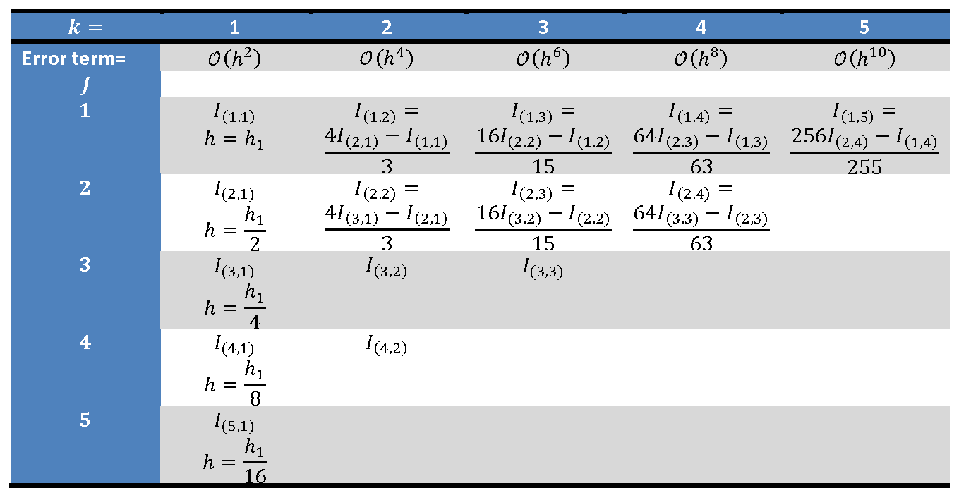
A stopping criterion for this algorithm can be set as:
![\[ \varepsilon_r=\left|\frac{I_{1,k}-I_{1,k-1}}{I_{1,k}}\right|\leq \varepsilon_s \]](https://engcourses-uofa.ca/wp-content/ql-cache/quicklatex.com-1bf040e278750bd276d3b72986260987_l3.png "Rendered by QuickLaTeX.com")
The following Mathematica code provides a procedural implementation of the Romberg’s method using the trapezoidal rule. The first procedure “IT[f,a,b,n]” provides the numerical estimate for the integral of from to with being the number of trapezoids. The “RI[f,a,b,k,n1]” procedure builds the Romberg’s method table shown above up to  columns.
  provides the number of subdivisions (number of trapezoids) in the first entry in the table
  .
.
View Mathematica Code
IT[f_, a_, b_, n_] := (h = (b - a)/n; Sum[(f[a + (i - 1)*h] + f[a + i*h])*h/2, {i, 1, n}])
RI[f_, a_, b_, k_,n1_] := (RItable = Table["N/A", {i, 1, k}, {j, 1, k}];
Do[RItable[[i, 1]] = IT[f, a, b, 2^(i - 1)*n1], {i, 1, k}];
  Do[RItable[[j, ik]] = (2^(2 (ik - 1)) RItable[[j + 1, ik - 1]] - RItable[[j, ik - 1]])/(2^(2 (ik - 1)) - 1), {ik, 2, k}, {j, 1,k - ik + 1}];
  ERtable =  Table[(RItable[[1, i + 1]] - RItable[[1, i]])/RItable[[1, i + 1]], {i, 1, k - 1}];
  {RItable, ERtable})
a = 0.0;
b = 2;
k=3;
n1=1;
f[x_] := E^x
Integrate[f[x], {x, a, b}]
s = RI[f, a, b, k,n1];
s[[1]] // MatrixForm
s[[2]] // MatrixForm
Example 1
As shown in the example above in the trapezoidal rule, when 71 trapezoids were used, the estimate for the integral of  from
from  to
to  was with an absolute error of
  . Using the Romberg’s method, find the depth starting with
  so that the estimate for the same integral has the same or less absolute error
  . Compare the number of computations required by the Romberg’s method to that required by the traditional trapezoidal rule to obtain an estimate with the same absolute error.
Solution
First, we will start with . For that, we will need to compute the integral numerically using the trapezoidal rule for a chosen and then for to fill in the entries and  in the Romberg’s method table.
Assuming , i.e., 1 trapezoid, the value of  . Assuming a trapezoid width of
  , i.e., two trapezoids on the interval, the value of
  . Using the Romberg table, the value of
  can be computed as:
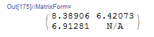
![\[ I_{1,2}=\frac{4I_{2,1}-I_{1,1}}{3}=6.42073 \]](https://engcourses-uofa.ca/wp-content/ql-cache/quicklatex.com-7c63844ebd5158e44b1d519a00a148ff_l3.png "Rendered by QuickLaTeX.com")
with a corresponding absolute error of  .
.
The output Romberg table with depth has the following form:
Next, to fill in the table up to depth , the value of  in the table needs to be calculated. This value corresponds to the calculation of the trapezoidal rule with a trapezoid width of
  , i.e., 4 trapezoids on the whole interval. Using the trapezoidal rule, we get
  . The remaining values in the Romberg table can be calculated as follows:
![\[\begin{split} I_{2,2}&=\frac{4I_{3,1}-I_{2,1}}{3}=\frac{4\times 6.52161-6.91281}{3}=6.39121\\ I_{1,3}&=\frac{16I_{2,2}-I_{1,2}}{15}=\frac{16\times 6.39121-6.42073}{15}=6.38924\\ \end{split} \]](https://engcourses-uofa.ca/wp-content/ql-cache/quicklatex.com-877ec4749d165e0524a75a2e8bca58f6_l3.png "Rendered by QuickLaTeX.com")
with the absolute error in  that is less than the specified error:
  . The output Romberg table with depth has the following form:
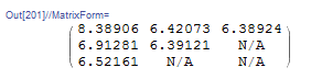
Number of Computations
For the same error, the traditional trapezoidal rule would have required 71 trapezoids. If we assume each trapezoid is one computation, the Romberg’s method requires computations of 1 trapezoid in , two trapezoids in , and 4 trapezoids in with a total of 7 corresponding computations. I.e., almost one tenth of the computational resources is required by the Romberg’s method in this example to produce the same level of accuracy!
The following Mathematica code was used to produce the above calculations.
View Mathematica CodeIT[f_, a_, b_, n_] := (h = (b - a)/n; Sum[(f[a + (i - 1)*h] + f[a + i*h])*h/2, {i, 1, n}])
RI[f_, a_, b_, k_, n1_] := (RItable = Table["N/A", {i, 1, k}, {j, 1, k}];
Do[RItable[[i, 1]] = IT[f, a, b, 2^(i - 1)*n1], {i, 1, k}];
Do[RItable[[j,ik]] = (2^(2 (ik - 1)) RItable[[j + 1, ik - 1]] - RItable[[j, ik - 1]])/(2^(2 (ik - 1)) - 1), {ik, 2, k}, {j, 1, k - ik + 1}];
ERtable = Table[(RItable[[1, i + 1]] - RItable[[1, i]])/RItable[[1, i + 1]], {i, 1, k - 1}];
{RItable, ERtable})
a = 0.0;
b = 2;
(*Depth of Romberg Table*)
k = 3;
n1 = 1;
f[x_] := E^x
Itrue = Integrate[f[x], {x, a, b}]
s = RI[f, a, b, k, n1];
s[[1]] // MatrixForm
s[[2]] // MatrixForm
ErrorTable = Table[If[RItable[[i, j]] == "N/A", "N/A", Abs[Itrue - RItable[[i, j]]]], {i, 1, Length[RItable]}, {j, 1, Length[RItable]}];
ErrorTable // MatrixForm
Example 2
Consider the integral:
![\[ I=\int_{0}^{1.5}\! 2 + 2 x + x^2 + \sin{(2 \pi x)} + \cos{(2 \pi \frac{x}{0.5})}\,\mathrm{d}x \]](https://engcourses-uofa.ca/wp-content/ql-cache/quicklatex.com-9afcfdaabc59330960b0dde2a4aa4672_l3.png "Rendered by QuickLaTeX.com")
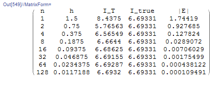
Using the trapezoidal rule, draw a table with the following columns: , , ,  , and
, and  , where is the number of trapezoids, is the width of each trapezoid, is the estimate using the trapezoidal rule, is the true value of the integral, and is the absolute value of the error. Use
  . Similarly, provide the Romberg table with depth
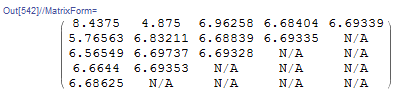
  . Compare the number of computations in each and the level of accuracy.
Solution
The true value of the integral can be computed using Mathematica as  . For the trapezoidal rule, the following Mathematica code is used to produce the required table for the specified values of :
IT[f_, a_, b_, n_] := (h = (b - a)/n;   Sum[(f[a + (i - 1)*h] + f[a + i*h])*h/2, {i, 1, n}])
a = 0.0;
b = 1.5;
f[x_] := 2 + 2 x + x^2 + Sin[2 Pi*x] + Cos[2 Pi*x/0.5]
Title = {"n", "h", "I_T", "I_true", "|E|"};
Ii = Table[{2^(i - 1), (b - a)/2^(i - 1), ss = IT[f, a, b, 2^(i - 1)], Itrue, Abs[Itrue - ss]}, {i, 1, 8}];
Ii = Prepend[Ii, Title];
Ii // MatrixForm
The table shows that with 128 subdivisions, the value of the absolute error is 0.00011.
For the Romberg table, the code developed above is used to produce the following table:
View Mathematica CodeIT[f_, a_, b_, n_] := (h = (b - a)/n; Sum[(f[a + (i - 1)*h] + f[a + i*h])*h/2, {i, 1, n}])
RI[f_, a_, b_, k_, n1_] := (RItable = Table["N/A", {i, 1, k}, {j, 1, k}];
Do[RItable[[i, 1]] = IT[f, a, b, 2^(i - 1)*n1], {i, 1, k}];
Do[RItable[[j, ik]] = (2^(2 (ik - 1)) RItable[[j + 1, ik - 1]] - RItable[[j, ik - 1]])/(2^(2 (ik - 1)) - 1), {ik, 2, k}, {j, 1, k - ik + 1}];
ERtable = Table[(RItable[[1, i + 1]] - RItable[[1, i]])/ RItable[[1, i + 1]], {i, 1, k - 1}];
{RItable, ERtable})
a = 0.0;
b = 1.5;
k = 5;
n1 = 1;
f[x_] := 2 + 2 x + x^2 + Sin[2 Pi*x] + Cos[2 Pi*x/0.5]
Itrue = Integrate[f[x], {x, a, b}]
s = RI[f, a, b, k, n1];
s[[1]] // MatrixForm
s[[2]] // MatrixForm
ErrorTable = Table[If[RItable[[i, j]] == "N/A", "N/A", Abs[Itrue - RItable[[i, j]]]], {i, 1, Length[RItable]}, {j, 1, Length[RItable]}];
ErrorTable // MatrixForm
The corresponding errors are given in the following table:
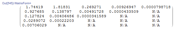
Comparing the table produced for the traditional trapezoidal method and that produced by the Romberg’s method reveals how powerful the Romberg’s method is. The Romberg table utilizes only the first 5 entries (up to  ) in the traditional trapezoidal method table and then using a few calculations according to the Romberg’s method equation, produces a value with an absolute error of 0.0000799 which is less than that with traditional trapezoidal rule with
  .
.
Gauss Quadrature
The Gauss integration scheme is a very efficient method to perform numerical integration over intervals. In fact, if the function to be integrated is a polynomial of an appropriate degree, then the Gauss integration scheme produces exact results. The Gauss integration scheme has been implemented in almost every finite element analysis software due to its simplicity and computational efficiency. This section outlines the basic principles behind the Gauss integration scheme. For its application to the finite element analysis method, please visit this section.
Introduction
Gauss quadrature aims to find the “least” number of fixed points to approximate the integral of a function ![f:[-1,1]\rightarrow \mathbb{R}](https://engcourses-uofa.ca/wp-content/ql-cache/quicklatex.com-b44be0e881a5cad1d59dd1a3856eeac5_l3.png "Rendered by QuickLaTeX.com") such that:
such that:
![\[ I=\int_{-1}^{1} \! f\,\mathrm{d}x \approx \sum_{i=1}^n w_i f(x_i) \]](https://engcourses-uofa.ca/wp-content/ql-cache/quicklatex.com-9adaa33f02ecc5f5cfa25d8a6d023502_l3.png "Rendered by QuickLaTeX.com")
where ![\forall 1\leq i\leq n:x_i\in[a,b]](https://engcourses-uofa.ca/wp-content/ql-cache/quicklatex.com-9ef1d4c6b91fba3faf45c80cdca61174_l3.png "Rendered by QuickLaTeX.com") and
and  . Also,
  is called an integration point and
  is called the associated weight. The number of integration points and the associated weights are chosen according to the complexity of the function to be integrated. Since a general polynomial of degree
  has coefficients, it is possible to find a Gauss integration scheme with number of integration points and number of associated weights to exactly integrate that polynomial function on the interval
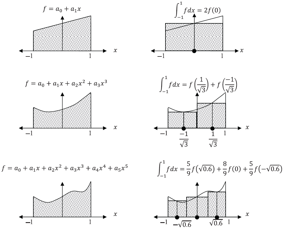
 ![[-1,1]](https://engcourses-uofa.ca/wp-content/ql-cache/quicklatex.com-4a7430a5619e08a23c430423c1376967_l3.png "Rendered by QuickLaTeX.com") . The following figure illustrates the concept of using the Gauss integration points to calculate the area under the curve for polynomials. In the following sections, the required number of integration points for particular polynomials are presented.
. The following figure illustrates the concept of using the Gauss integration points to calculate the area under the curve for polynomials. In the following sections, the required number of integration points for particular polynomials are presented.
Gauss Integration for Polynomials of the 1st, 3rd and 5th Degrees
Affine Functions (First-Degree Polynomials): One Integration Point
For a first-degree polynomial,  , therefore, , so, 1 integration point is sufficient as will be shown here. Consider
  with
with  , then:
![\[ \int_{-1}^{1} \! ax+b\,\mathrm{d}x=2b+a\frac{x^2}{2}\bigg|_{-1}^1=2b=2f(0) \]](https://engcourses-uofa.ca/wp-content/ql-cache/quicklatex.com-42598724c9bce16915b2fe2234930c73_l3.png "Rendered by QuickLaTeX.com")
So, for functions that are very close to being affine, a numerical integration scheme with 1 integration point that is  with an associated weight of 2 can be employed. In other words, a one-point numerical integration scheme has the form:
![\[ I=\int_{-1}^{1} \! f\,\mathrm{d}x \approx 2 f(0) \]](https://engcourses-uofa.ca/wp-content/ql-cache/quicklatex.com-140ab06e1479f22d19a13f9153c729ec_l3.png "Rendered by QuickLaTeX.com")
Third-Degree Polynomials: Two Integration Points
For a third-degree polynomial,  , therefore, , so, 2 integration points are sufficient as will be shown here. Consider
  , then:
![\[ \int_{-1}^{1} \! a_0+a_1x+a_2x^2+a_3x^3\,\mathrm{d}x=2a_0+2\frac{a_2}{3} \]](https://engcourses-uofa.ca/wp-content/ql-cache/quicklatex.com-588d17912294b3e4b0fce33b8eee7a44_l3.png "Rendered by QuickLaTeX.com")
Assuming 2 integration points in the Gauss integration scheme yields:
![\[ \int_{-1}^{1} \! a_0+a_1x+a_2x^2+a_3x^3\,\mathrm{d}x=w_1(a_0+a_1x_1+a_2x_1^2+a_3x_1^3)+w_2(a_0+a_1x_2+a_2x_2^2+a_3x_2^3) \]](https://engcourses-uofa.ca/wp-content/ql-cache/quicklatex.com-9fbfd96968875652a0d3f5b3146b9fd9_l3.png "Rendered by QuickLaTeX.com")
For the Gauss integration scheme to yield accurate results, the right-hand sides of the two equations above need to be equal for any choice of a cubic function. Therefore the multipliers of  ,
,  ,
,  , and
, and  should be the same. So, four equations in four unknowns can be written as follows:
![\[ \begin{split} w_1+w_2&=2\\ w_1x_1+w_2x_2&=0\\ w_1x_1^2+w_2x_2^2&=\frac{2}{3}\\ w_1x_1^3+w_2x_2^3&=0 \end{split} \]](https://engcourses-uofa.ca/wp-content/ql-cache/quicklatex.com-7acd5b30af7e2c531a452cc86be7a1af_l3.png "Rendered by QuickLaTeX.com")
The solution to the above four equations yields  ,
,  ,
,  . The Mathematica code below forms the above equations and solves them:
View Mathematica Code
f = a0 + a1*x + a2*x^2 + a3*x^3;
I1 = Integrate[f, {x, -1, 1}]
I2 = w1*(f /. x -> x1) + w2*(f /. x -> x2)
Eq1 = Coefficient[I1 - I2, a0]
Eq2 = Coefficient[I1 - I2, a1]
Eq3 = Coefficient[I1 - I2, a2]
Eq4 = Coefficient[I1 - I2, a3]
Solve[{Eq1 == 0, Eq2 == 0, Eq3 == 0, Eq4 == 0}, {x1, x2, w1, w2}]
So, for functions that are very close to being cubic, the following numerical integration scheme with 2 integration points can be employed:
![\[ I=\int_{-1}^{1} \! f\,\mathrm{d}x \approx f\left(\frac{-1}{\sqrt{3}}\right)+f\left(\frac{1}{\sqrt{3}}\right) \]](https://engcourses-uofa.ca/wp-content/ql-cache/quicklatex.com-4e2e3cd0f4f9a394e1dd4cc87ad07a36_l3.png "Rendered by QuickLaTeX.com")
Fifth-Degree Polynomials: Three Integration Points
For a fifth-degree polynomial,  , therefore,
  , so, 3 integration points are sufficient to exactly integrate a fifth-degree polynomial. Consider
  , then:
![\[ \int_{-1}^{1} \! a_0+a_1x+a_2x^2+a_3x^3+a_4x^4+a_5x^5\,\mathrm{d}x=2a_0+2\frac{a_2}{3}+2\frac{a_4}{5} \]](https://engcourses-uofa.ca/wp-content/ql-cache/quicklatex.com-d953ea0f7acca04c96dff423188e29a3_l3.png "Rendered by QuickLaTeX.com")
Assuming 3 integration points in the Gauss integration scheme yields:
![\[\begin{split} \int_{-1}^{1} \! a_0+a_1x+a_2x^2+a_3x^3\,\mathrm{d}x&=w_1(a_0+a_1x_1+a_2x_1^2+a_3x_1^3)+w_2(a_0+a_1x_2+a_2x_2^2+a_3x_2^3)\\ &+w_3(a_0+a_1x_3+a_2x_3^2+a_3x_3^3) \end{split} \]](https://engcourses-uofa.ca/wp-content/ql-cache/quicklatex.com-3e8dbbfe0f4a5782573069a6b6a8c2d5_l3.png "Rendered by QuickLaTeX.com")
For the Gauss integration scheme to yield accurate results, the right-hand sides of the two equations above need to be equal for any choice of a fifth-order polynomial function. Therefore the multipliers of , , , ,  , and
, and  should be the same. So, six equations in six unknowns can be written as follows:
![\[ \begin{split} w_1+w_2+w_3&=2\\ w_1x_1+w_2x_2+w_3x_3&=0\\ w_1x_1^2+w_2x_2^2+w_3x_3^2&=\frac{2}{3}\\ w_1x_1^3+w_2x_2^3+w_3x_3^3&=0\\ w_1x_1^4+w_2x_2^4+w_3x_3^4&=\frac{2}{5}\\ w_1x_1^5+w_2x_2^5+w_3x_3^5&=0 \end{split} \]](https://engcourses-uofa.ca/wp-content/ql-cache/quicklatex.com-079fb8f3210a619d9848a61fc7bd8051_l3.png "Rendered by QuickLaTeX.com")
The solution to the above six equations yields  ,
,  ,
,  ,
,  ,
,  , and
, and  . The Mathematica code below forms the above equations and solves them:
View Mathematica Code
f = a0 + a1*x + a2*x^2 + a3*x^3 + a4*x^4 + a5*x^5;
I1 = Integrate[f, {x, -1, 1}]
I2 = w1*(f /. x -> x1) + w2*(f /. x -> x2) + w3*(f /. x -> x3)
Eq1 = Coefficient[I1 - I2, a0]
Eq2 = Coefficient[I1 - I2, a1]
Eq3 = Coefficient[I1 - I2, a2]
Eq4 = Coefficient[I1 - I2, a3]
Eq5 = Coefficient[I1 - I2, a4]
Eq6 = Coefficient[I1 - I2, a5]
Solve[{Eq1 == 0, Eq2 == 0, Eq3 == 0, Eq4 == 0, Eq5 == 0, Eq6 == 0}, {x1, x2, x3, w1, w2, w3}]
So, for functions that are very close to being fifth-order polynomials, the following numerical integration scheme with 3 integration points can be employed:
![\[ I=\int_{-1}^{1} \! f\,\mathrm{d}x \approx \frac{5}{9}f\left(-\sqrt{\frac{3}{5}}\right)+\frac{8}{9}f(0)+\frac{5}{9}f\left(\sqrt{\frac{3}{5}}\right) \]](https://engcourses-uofa.ca/wp-content/ql-cache/quicklatex.com-967f03f737cbcb8b546f3755a1759bef_l3.png "Rendered by QuickLaTeX.com")
Seventh-Degree Polynomial: Four Integration Points
For a seventh-degree polynomial,  , therefore, , so, 4 integration points are sufficient to exactly integrate a seventh-degree polynomial. Following the procedure outlined above, the integration points along with the associated weight:
![\[\begin{split} x_1=-0.861136 \qquad w_1=0.347855\\ x_2=-0.339981 \qquad w_2=0.652145\\ x_3=0.339981 \qquad w_3=0.652145\\ x_4=0.861136 \qquad w_4=0.347855 \end{split} \]](https://engcourses-uofa.ca/wp-content/ql-cache/quicklatex.com-45e63564a6dd5756605d5fb69bb89c29_l3.png "Rendered by QuickLaTeX.com")
So, for functions that are very close to being seventh-order polynomials, the following numerical integration scheme with 4 integration points can be employed:
![\[\begin{split} I&=\int_{-1}^{1} \! f\,\mathrm{d}x\\ & \approx 0.347855f(-0.861136)+0.652145f(-0.339981)\\ & +0.652145f(0.339981)+0.347855f(0.861136) \end{split} \]](https://engcourses-uofa.ca/wp-content/ql-cache/quicklatex.com-7ef1e067e795fffd6bb0b612e96f6185_l3.png "Rendered by QuickLaTeX.com")
The following is the Mathematica code used to find the above integration points and corresponding weights.
View Mathematica Codef = a0 + a1*x + a2*x^2 + a3*x^3 + a4*x^4 + a5*x^5 + a6*x^6 + a7*x^7;
I1 = Integrate[f, {x, -1, 1}]
I2 = w1*(f /. x -> x1) + w2*(f /. x -> x2) + w3*(f /. x -> x3) + w4*(f /. x -> x4)
Eq1 = Coefficient[I1 - I2, a0]
Eq2 = Coefficient[I1 - I2, a1]
Eq3 = Coefficient[I1 - I2, a2]
Eq4 = Coefficient[I1 - I2, a3]
Eq5 = Coefficient[I1 - I2, a4]
Eq6 = Coefficient[I1 - I2, a5]
Eq7 = Coefficient[I1 - I2, a6]
Eq8 = Coefficient[I1 - I2, a7]
a = Solve[{Eq1 == 0, Eq2 == 0, Eq3 == 0, Eq4 == 0, Eq5 == 0, Eq6 == 0, Eq7 == 0, Eq8 == 0}, {x1, x2, x3, w1, w2, w3, x4, w4}]
Chop[N[a[[1]]]]
Ninth-Degree Polynomial: Five Integration Points
For a ninth-degree polynomial,  , therefore,
  , so, 5 integration points are sufficient to exactly integrate a ninth-degree polynomial. Following the procedure outlined above, the integration points along with the associated weight:
![\[\begin{split} x_1=-0.90618 \qquad w_1=0.236927\\ x_2=-0.538469 \qquad w_2=0.478629\\ x_3=0 \qquad w_3=0.568889\\ x_4=0.538469 \qquad w_4=0.478629\\ x_5=0.90618 \qquad w_5=0.236927 \end{split} \]](https://engcourses-uofa.ca/wp-content/ql-cache/quicklatex.com-70074209cd7d5d45f3ad78d9e28a4f31_l3.png "Rendered by QuickLaTeX.com")
So, for functions that are very close to being ninth-order polynomials, the following numerical integration scheme with 5 integration points can be employed:
![\[\begin{split} I&=\int_{-1}^{1} \! f\,\mathrm{d}x\\ & \approx 0.236927f(-0.90618)+0.478629f(-0.538469)\\ & +0.568889f(0)+0.478629f(0.538469)\\ & + 0.236927 f(0.90618) \end{split} \]](https://engcourses-uofa.ca/wp-content/ql-cache/quicklatex.com-053256c5108eadf390d18e603028c575_l3.png "Rendered by QuickLaTeX.com")
The following is the Mathematica code used to find the above integration points and corresponding weights.
View Mathematica Codef = a0 + a1*x + a2*x^2 + a3*x^3 + a4*x^4 + a5*x^5 + a6*x^6 + a7*x^7 + a8*x^8 + a9*x^9;
I1 = Integrate[f, {x, -1, 1}]
I2 = w1*(f /. x -> x1) + w2*(f /. x -> x2) + w3*(f /. x -> x3) + w4*(f /. x -> x4) + w5*(f /. x -> x5)
Eq1 = Coefficient[I1 - I2, a0]
Eq2 = Coefficient[I1 - I2, a1]
Eq3 = Coefficient[I1 - I2, a2]
Eq4 = Coefficient[I1 - I2, a3]
Eq5 = Coefficient[I1 - I2, a4]
Eq6 = Coefficient[I1 - I2, a5]
Eq7 = Coefficient[I1 - I2, a6]
Eq8 = Coefficient[I1 - I2, a7]
Eq9 = Coefficient[I1 - I2, a8]
Eq10 = Coefficient[I1 - I2, a9]
a = Solve[{Eq1 == 0, Eq2 == 0, Eq3 == 0, Eq4 == 0, Eq5 == 0, Eq6 == 0, Eq7 == 0, Eq8 == 0, Eq9 == 0, Eq10 == 0}, {x1, x2, x3, w1, w2, w3, x4, w4, x5, w5}]
Chop[N[a[[1]]]]
Eleventh-Degree Polynomial: Six Integration Points
For an eleventh-degree polynomial,  , therefore,
  , so, 6 integration points are sufficient to exactly integrate an eleventh-degree polynomial. Following the procedure outlined above, the integration points along with the associated weight:
![\[\begin{split} x_1=-0.93247 \qquad w_1=0.171324\\ x_2=-0.661209 \qquad w_2=0.360762\\ x_3=-0.238619 \qquad w_3=0.467914\\ x_4=0.238619 \qquad w_4=0.467914\\ x_5=0.661209 \qquad w_5=0.360762\\ x_6=0.93247 \qquad w_6=0.171324\\ \end{split} \]](https://engcourses-uofa.ca/wp-content/ql-cache/quicklatex.com-a0030a33255bb167e53520bcd05a6476_l3.png "Rendered by QuickLaTeX.com")
So, for functions that are very close to being eleventh-order polynomials, the following numerical integration scheme with 6 integration points can be employed:
![\[\begin{split} I&=\int_{-1}^{1} \! f\,\mathrm{d}x\\ & \approx 0.171324f(-0.93247 )+0.360762f(-0.661209 )\\ & +0.467914f(-0.238619)+0.467914f(0.238619)\\ & + 0.360762f(0.661209 )+0.171324f(0.93247 ) \end{split} \]](https://engcourses-uofa.ca/wp-content/ql-cache/quicklatex.com-d2bf620ef2d07461c9ea37101ea7f555_l3.png "Rendered by QuickLaTeX.com")
The following is the Mathematica code used to find the above integration points and corresponding weights. Note that symmetry was employed to reduce the number of equations.
View Mathematica Codef = a0 + a1*x + a2*x^2 + a3*x^3 + a4*x^4 + a5*x^5 + a6*x^6 + a7*x^7 + a8*x^8 + a9*x^9 + a10*x^10 + a11*x^11;
I1 = Integrate[f, {x, -1, 1}]
I2 = w1*(f /. x -> x1) + w2*(f /. x -> x2) + w3*(f /. x -> x3) +
w3*(f /. x -> -x3) + w2*(f /. x -> -x2) + w1*(f /. x -> -x1)]
Eq1 = Coefficient[I1 - I2, a0]
Eq3 = Coefficient[I1 - I2, a2]
Eq5 = Coefficient[I1 - I2, a4]
Eq7 = Coefficient[I1 - I2, a6]
Eq9 = Coefficient[I1 - I2, a8]
Eq11 = Coefficient[I1 - I2, a10]
a = Solve[{Eq1 == 0, Eq3 == 0, Eq5 == 0, Eq7 == 0, Eq9 == 0, Eq11 == 0}, {x1, x2, x3, w1, w2, w3}]
Chop[N[a[[1]]]]
Implementation of Gauss Quadrature
Gauss quadrature is very easy to implement and provides very accurate results with very few computations. However, one drawback is that it is not applicable to data obtained experimentally as the values of the function at the specific integration points would not be necessarily available. In order to implement the Gauss integration scheme in Mathematica, first, the following table is created which contains the integration points and the corresponding weights. Row number contains the Gauss integration scheme with  integration points. Then, a procedure is created in Mathematica whose input is a function , and the requested number of integration points. The procedure then calls the appropriate row in the “GaussTable” and calculates the weighted sum of the function evaluated at the appropriate integration points.
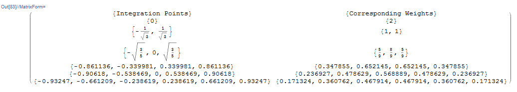
Clear[f, x]
GaussTable = {{{"Integration Points"}, {"Corresponding Weights"}}, {{0}, {2}}, {{-1/Sqrt[3], 1/Sqrt[3]}, {1, 1}}, {{-Sqrt[3/5], 0, Sqrt[3/5]}, {5/9, 8/9, 5/9}}, {{-0.861136, -0.339981, 0.339981, 0.861136}, {0.347855, 0.652145, 0.652145, 0.347855}}, {{-0.90618, -0.538469, 0, 0.538469, 0.90618}, {0.236927, 0.478629, 0.568889, 0.478629, 0.236927}}, {{-0.93247, -0.661209, -0.238619, 0.238619, 0.661209, 0.93247}, {0.171324, 0.360762, 0.467914, 0.467914, 0.360762,  0.171324}}};
GaussTable // MatrixForm
IG[f_, n_] := Sum[GaussTable[[n + 1, 2, i]]*f[GaussTable[[n + 1, 1, i]]], {i, 1, n}]
f[x_] := x^9 + x^8
IG[f, 5.0]
Example
Calculate the exact integral of  on the interval and find the relative error if a Gauss 1, 2, 3, and 4 integration points scheme is used. Also, calculate the number of rectangles required by the midpoint rule of the rectangle method to produce an error similar to that produced by the 3 point integration scheme, then evaluate the integral using the midpoint rule of the rectangle method with the obtained number of rectangles.
Solution
The exact integral is given by:
![\[ I=\int_{-1}^{1}\!\cos{x}\,\mathrm{d}x=\sin{(1)}-\sin{(-1)}=1.68294 \]](https://engcourses-uofa.ca/wp-content/ql-cache/quicklatex.com-411d1a03d3721da1944a209774229637_l3.png "Rendered by QuickLaTeX.com")
Employing a Gauss integration scheme with one integration point yields:
![\[\begin{split} I_1&=w_1\cos{x_1}=2 \cos{(0)}=2\\ E_r&=\frac{1.68294-2}{1.68294}=-0.1884 \end{split} \]](https://engcourses-uofa.ca/wp-content/ql-cache/quicklatex.com-f871bfb56b2deff0815944cefebe41b9_l3.png "Rendered by QuickLaTeX.com")
Employing a Gauss integration scheme with two integration points yields:
![\[ \begin{split} I_2&=w_1\cos{x_1}+w_2\cos{x_2}=\cos{\left(\frac{-1}{\sqrt{3}}\right)}+\cos{\left(\frac{1}{\sqrt{3}}\right)}=1.67582\\ E_r&=\frac{1.68294-1.67582}{1.68294}=0.00422968 \end{split} \]](https://engcourses-uofa.ca/wp-content/ql-cache/quicklatex.com-32caa2476d3464e03e8141b99e407065_l3.png "Rendered by QuickLaTeX.com")
Employing a Gauss integration scheme with three integration points yields:
![\[\begin{split} I_3&=w_1\cos{x_1}+w_2\cos{x_2}+w_3\cos{x_3}=\frac{5}{9}\cos{\left(-\sqrt{\frac{3}{5}}\right)}+\frac{8}{9}\cos{(0)}+\frac{5}{9}\cos{\left(\sqrt{\frac{3}{5}}\right)}=1.683\\ E_r&=\frac{1.68294-1.683}{1.68294}=-0.0003659 \end{split} \]](https://engcourses-uofa.ca/wp-content/ql-cache/quicklatex.com-b5c7c72a6720733f903c8511a9eaeb5c_l3.png "Rendered by QuickLaTeX.com")
Employing a Gauss integration scheme with four integration points yields:
![\[\begin{split} I_4&=w_1\cos{x_1}+w_2\cos{x_2}+w_3\cos{x_3}+w_4\cos{x_4}\\ &= 0.347855\cos(-0.861136)+0.652145\cos(-0.339981)\\ &+0.652145\cos(0.339981)+0.347855\cos(0.861136)\\ &=1.68294\\ E_r&=\frac{1.68294-1.68294}{1.68294}=0 \end{split} \]](https://engcourses-uofa.ca/wp-content/ql-cache/quicklatex.com-3ba045ee209d628ff6bab12db3ba324a_l3.png "Rendered by QuickLaTeX.com")
Using a three point integration scheme yielded an error of:
![\[ |E|=|1.68294-1.683| = |-0.00006|=0.00006 \]](https://engcourses-uofa.ca/wp-content/ql-cache/quicklatex.com-5db8c84e888ed0ed9ececfd183ddeda3_l3.png "Rendered by QuickLaTeX.com")
Equating the upper bound for the error in the midpoint rule to the error produced by a three-point Gauss integration scheme yields:
![\[ \max_{\xi\in[a,b]}|f''(\xi)| (b-a)\frac{h^2}{24}=0.00006 \]](https://engcourses-uofa.ca/wp-content/ql-cache/quicklatex.com-f6df0dbe7737379b80e42192bbaf2bf2_l3.png "Rendered by QuickLaTeX.com")
With  , and
, and ![\max_{\xi\in[a,b]}|f''(\xi)|=1](https://engcourses-uofa.ca/wp-content/ql-cache/quicklatex.com-19a68e3a4230df3f1dd7ed409251ea7a_l3.png "Rendered by QuickLaTeX.com") . Therefore:
. Therefore:
![\[ h=\sqrt{\frac{0.00006\times 24}{2}}=0.02683 \]](https://engcourses-uofa.ca/wp-content/ql-cache/quicklatex.com-5bc61f14f58f49f7447da4273559c8e8_l3.png "Rendered by QuickLaTeX.com")
Therefore, the required number of rectangles is:
![\[ n=\frac{b-a}{h}=\frac{2}{0.02683}\approx 75 \]](https://engcourses-uofa.ca/wp-content/ql-cache/quicklatex.com-a2c8417b5e8a49b2f6b840f81c4dfc4e_l3.png "Rendered by QuickLaTeX.com")
With 75 rectangles the rectangle method yields an integral of  . It is important to note how accurate the Gauss integration scheme is compared to the rectangle method. For this example, it would take 75 divisions (equivalent to 75 integration points) to reach an accuracy similar to the Gauss integration scheme with only 3 points!
Clear[f, x, I2]
GaussTable = {{{"Integration Points"}, {"Corresponding Weights"}}, {{0}, {2}}, {{-1/Sqrt[3], 1/Sqrt[3]}, {1, 1}}, {{-Sqrt[3/5], 0,  Sqrt[3/5]}, {5/9, 8/9, 5/9}}, {{-0.861136, -0.339981, 0.339981, 0.861136}, {0.347855, 0.652145, 0.652145, 0.347855}}, {{-0.90618, -0.538469, 0, 0.538469, 0.90618}, {0.236927, 0.478629, 0.568889, 0.478629, 0.236927}}, {{-0.93247, -0.661209, -0.238619, 0.238619, 0.661209, 0.93247}, {0.171324, 0.360762, 0.467914, 0.467914, 0.360762,  0.171324}}};
GaussTable // MatrixForm
IG[f_, n_] := Sum[GaussTable[[n + 1, 2, i]]*f[GaussTable[[n + 1, 1, i]]], {i, 1,  n}];
f[x_] := Cos[x]
Iexact = Integrate[Cos[x], {x, -1, 1.0}]
Itable = Table[{i, N[IG[f, i]], (Iexact - IG[f, i])/Iexact}, {i, 1, 6}];
Title = {"Number of Integration Points",  "Numerical Integration Results", "Relative Error"};
Itable = Prepend[Itable, Title];
Itable // MatrixForm
h = Sqrt[0.00006*24/2/1]
n = Ceiling[2/h]
I2[f_, a_, b_, n_] := (h = (b - a)/n; Sum[f[a + (i - 1/2)*h]*h, {i, 1, n}])
I2[f, -1.0, 1, n]
Alternate Integration Limits
The Gauss integration scheme presented above applies to functions that are integrated over the interval . A simple change of variables can be used to allow integrating a function  where
where ![z\in[a,b]](https://engcourses-uofa.ca/wp-content/ql-cache/quicklatex.com-0df50d7343f494f1f6b9ccd9ee9ad2e8_l3.png "Rendered by QuickLaTeX.com") . In this case, the linear relationship between
. In this case, the linear relationship between  and can be expressed as:
![\[ \frac{z-a}{b-a}=\frac{x-(-1)}{1-(-1)}=\frac{x+1}{2} \]](https://engcourses-uofa.ca/wp-content/ql-cache/quicklatex.com-a4e8036b754090df2c3a9adf4d89d796_l3.png "Rendered by QuickLaTeX.com")
Therefore:
![\[ \mathrm{d}z=\frac{(b-a)}{2}\mathrm{d}x \]](https://engcourses-uofa.ca/wp-content/ql-cache/quicklatex.com-f9836330b8707aa688b748dbb82b62c9_l3.png "Rendered by QuickLaTeX.com")
Which means the integration can be converted from integrating over to integrating over as follows:
![\[ \int_{a}^b\! g(z)\,\mathrm{d}z=\int_{-1}^1\! g(z(x))\,\frac{(b-a)}{2}\mathrm{d}x \]](https://engcourses-uofa.ca/wp-content/ql-cache/quicklatex.com-e731dbb2e1323a067f1e06820d137c6e_l3.png "Rendered by QuickLaTeX.com")
where
![\[ z(x)=\frac{(b-a)(x+1)}{2}+a=\frac{(b-a)(x)+(b+a)}{2} \]](https://engcourses-uofa.ca/wp-content/ql-cache/quicklatex.com-a2eb9189c73b3eae97f56a6d18b8ef19_l3.png "Rendered by QuickLaTeX.com")
Therefore:
![\[ \int_{a}^b\! g(z)\,\mathrm{d}z=\int_{-1}^1\! g\left(\frac{(b-a)(x)+(b+a)}{2}\right)\,\frac{(b-a)}{2}\mathrm{d}x \]](https://engcourses-uofa.ca/wp-content/ql-cache/quicklatex.com-999c1e67f8514c0e6730c154173c936c_l3.png "Rendered by QuickLaTeX.com")
The integration can then proceed as per the weights and values of the integration points with given by:
![\[ f(x)=g\left(\frac{(b-a)(x)+(b+a)}{2}\right)\,\frac{(b-a)}{2} \]](https://engcourses-uofa.ca/wp-content/ql-cache/quicklatex.com-fca4daf91393ca0077d3f381637a9d9c_l3.png "Rendered by QuickLaTeX.com")
Example
Calculate the exact integral of  on the interval
 ![[0,3]](https://engcourses-uofa.ca/wp-content/ql-cache/quicklatex.com-6abe4233622b81d2a4a66682455d476b_l3.png "Rendered by QuickLaTeX.com") and find the absolute relative error if a Gauss 1, 2, 3, and 4 integration points scheme is used.
and find the absolute relative error if a Gauss 1, 2, 3, and 4 integration points scheme is used.
Solution
First, to differentiate between the given function limits, and the limits after changing variables, we will assume that the function is given in terms of as follows:
![\[ g(z)=ze^z \]](https://engcourses-uofa.ca/wp-content/ql-cache/quicklatex.com-858bc6a53c78f103e3b07adeab4afe3d_l3.png "Rendered by QuickLaTeX.com")
The exact integral is given by:
![\[ \int_{0}^3\!ze^z\,\mathrm{d}z=e^z(z-1)|_{z=0}^{z=3}=2e^3+1=41.1711 \]](https://engcourses-uofa.ca/wp-content/ql-cache/quicklatex.com-ce4db8a28a0474c748c94d68ca78b9ed_l3.png "Rendered by QuickLaTeX.com")
Using a linear change of variables  we have:
Therefore:
![\[ \int_{0}^3\! ze^z\,\mathrm{d}z=\int_{-1}^1\! g\left(\frac{3x+3}{2}\right)\frac{3}{2}\,\mathrm{d}x=\int_{-1}^1\! \left(\frac{(3x+3)}{2}\right)e^{\left(\frac{(3x+3)}{2}\right)}\frac{3}{2}\,\mathrm{d}x \]](https://engcourses-uofa.ca/wp-content/ql-cache/quicklatex.com-37ca0cacd730f85190fc2979dd31d506_l3.png "Rendered by QuickLaTeX.com")
Employing a Gauss integration scheme with one integration point yields:
![\[\begin{split} I_1&=w_1f(x_1)=2 f(0)=2 \left(\frac{(3(0)+3)}{2}\right)e^{\left(\frac{(3(0)+3)}{2}\right)}\frac{3}{2}=20.1676\\ E_r&=\frac{41.1711-20.1676}{41.1711}=0.51 \end{split} \]](https://engcourses-uofa.ca/wp-content/ql-cache/quicklatex.com-02ccecaf3cdb38d2b5abf1337894e136_l3.png "Rendered by QuickLaTeX.com")
Employing a Gauss integration scheme with two integration points yields:
![\[ \begin{split} I_2&=w_1f(x_1)+w_2f(x_2)\\ &=\left(\frac{(3\left(-\sqrt{\frac{1}{3}}\right)+3)}{2}\right)e^{\left(\frac{(3\left(-\sqrt{\frac{1}{3}}\right)+3)}{2}\right)}\frac{3}{2}+\left(\frac{(3\left(\sqrt{\frac{1}{3}}\right)+3)}{2}\right)e^{\left(\frac{(3\left(\sqrt{\frac{1}{3}}\right)+3)}{2}\right)}\frac{3}{2}=39.607\\ E_r&=\frac{41.1711-39.607}{41.1711}=0.038 \end{split} \]](https://engcourses-uofa.ca/wp-content/ql-cache/quicklatex.com-c2c91ccc3a1473df0ed31f907069b512_l3.png "Rendered by QuickLaTeX.com")
Employing a Gauss integration scheme with three integration points yields:
![\[\begin{split} I_3&=w_1f(x_1)+w_2f(x_2)+w_3f(x_3)=\frac{5}{9}f(x_1)+\frac{8}{9}f(x_2)+\frac{5}{9}f(x_3)=41.1313\\ E_r&=\frac{41.1711-41.1313}{41.1711}=0.0009657 \end{split} \]](https://engcourses-uofa.ca/wp-content/ql-cache/quicklatex.com-6b6e006b0964309110ddff2e1e999dbc_l3.png "Rendered by QuickLaTeX.com")
where,
![\[\begin{split} f(x_1)&=f(-\sqrt{0.6})=\left(\frac{(3(-\sqrt{0.6})+3)}{2}\right)e^{\left(\frac{(3(-\sqrt{0.6})+3)}{2}\right)}\frac{3}{2}\\ f(x_2)&=f(0)=\left(\frac{(3(0)+3)}{2}\right)e^{\left(\frac{(3(0)+3)}{2}\right)}\frac{3}{2}\\ f(x_3)&=f(\sqrt{0.6})=\left(\frac{(3(\sqrt{0.6})+3)}{2}\right)e^{\left(\frac{(3(\sqrt{0.6})+3)}{2}\right)}\frac{3}{2} \end{split} \]](https://engcourses-uofa.ca/wp-content/ql-cache/quicklatex.com-4c74eadf66b3899cd900a882a0dea8f3_l3.png "Rendered by QuickLaTeX.com")
In the following Mathematica code, the procedure IGAL applies the Gauss integration scheme with integration points to a function on the interval
View Mathematica Code
GaussTable = {{{"Integration Points"}, {"Corresponding Weights"}}, {{0}, {2}}, {{-1/Sqrt[3], 1/Sqrt[3]}, {1, 1}}, {{-Sqrt[3/5], 0,  Sqrt[3/5]}, {5/9, 8/9, 5/9}}, {{-0.861136, -0.339981, 0.339981,  0.861136}, {0.347855, 0.652145, 0.652145,  0.347855}}, {{-0.90618, -0.538469, 0, 0.538469, 0.90618}, {0.236927, 0.478629, 0.568889, 0.478629,  0.236927}}, {{-0.93247, -0.661209, -0.238619, 0.238619, 0.661209,      0.93247}, {0.171324, 0.360762, 0.467914, 0.467914, 0.360762,      0.171324}}};
GaussTable // MatrixForm
IGAL[f_, n_, a_, b_] := Sum[(b - a)/2*GaussTable[[n + 1, 2, i]]*f[(b - a)/2*(GaussTable[[n + 1, 1, i]] + 1) + a], {i, 1, n}]
f[x_] := x*E^x
Iexact = Integrate[f[x], {x, 0., 3}]
Itable = Table[{i, N[IGAL[f, i, 0, 3]], (Iexact - IGAL[f, i, 0, 3])/Iexact}, {i, 1, 6}];
Title = {"Number of Integration Points",  "Numerical Integration Results", "Relative Error"};
Itable = Prepend[Itable, Title];
Itable // MatrixForm
Problems
- Consider the following integral
![\[ \int_{0}^4\! 1-e^{-x}\,\mathrm{d}x \]](https://engcourses-uofa.ca/wp-content/ql-cache/quicklatex.com-d097774e17448c3a6b8b69fcf5b7fad3_l3.png "Rendered by QuickLaTeX.com")
- Evaluate the integral analytically.
- Evaluate the integral using the trapezoidal rule with ,
 , and
, and  . For each case, calculate the relative error.
 - Evaluate the integral using the Simpson’s 1/3 rule with , , and . For each case, calculate the relative error.
- Evaluate the integral using the Simpson’s 3/8 rule with , , and . For each case, calculate the relative error.
- Comment on the accuracy of the methods used above.
- A transportation engineering study requires calculating the number of cars through an intersection travelling during morning rush hour. The following table provides the number of cars that pass every 4 minutes at particular times during that period:
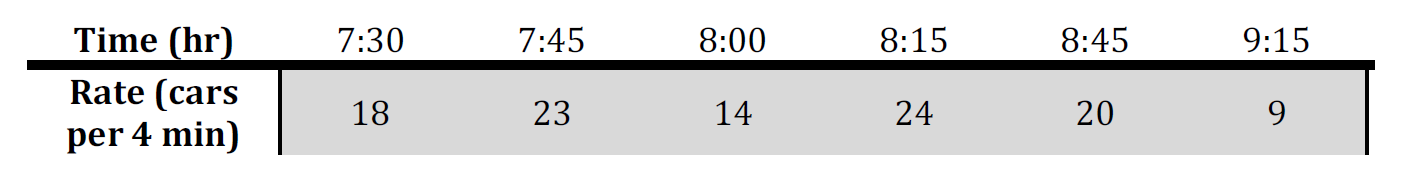
- Find the corresponding rate of cars through the intersection per minute
- By integrating the rate of cars per minute over the interval from 7:30 a.m. to 9:15 a.m., find the total number of cars that pass through the intersection. Use an appropriate integration method and justify its use.
- Consider the following integral
![\[ \int_{0}^3\!xe^{2x}\,\mathrm{d}x \]](https://engcourses-uofa.ca/wp-content/ql-cache/quicklatex.com-535ca72a59316de993e710b27f9799a8_l3.png "Rendered by QuickLaTeX.com")
- Evaluate the integral analytically.
- Evaluate the integral using the Romberg’s method with a depth such that
 .
. - Evaluate the integral using the Gauss integration scheme with 1, 2, 3, and 4 integration point. Calculate the relative error in each case.
- Comment on the number of integration points required to achieve an acceptable accuracy.
- Consider the following integral
![\[ \mbox{erf}(a)=\frac{2}{\sqrt{\pi}}\int_{0}^{a}e^{-x^2}\,\mathrm{d}x \]](https://engcourses-uofa.ca/wp-content/ql-cache/quicklatex.com-9b25370be71f518c58c2ecf1c3b77b40_l3.png "Rendered by QuickLaTeX.com")
with

- Use the built-in numerical integration “NIntegrate” function to calculate an approximation to the true value of the integral. Consider this to be the true value.
- Evaluate the integral using the Gauss integration scheme with 1, 2, 3, and 4 integration point. Calculate the relative error in each case.
- The amount of mass transported via a pipe over a period of time can be computed as:
![\[ M=\int_{t_1}^{t_2}\!Q(t)c(t)\,\mathrm{d}t \]](https://engcourses-uofa.ca/wp-content/ql-cache/quicklatex.com-73e5a94145daeabc41ec5e846b72f60e_l3.png "Rendered by QuickLaTeX.com")
where
 is the mass in
  ,
,  is the initial time in minutes,
  is the final time in minutes,
  is the flow rate in
  , and
, and  is the concentration in
  . The following functional representations define the temporal variations in flow and concentration:
![\[\begin{split} Q(t)&=9+5(\cos{(0.4t)} )^2\\ c(t)&=5e^{-0.5t}+2e^{0.15t} \end{split} \]](https://engcourses-uofa.ca/wp-content/ql-cache/quicklatex.com-d598f01e981b6bbfee91c37d73c3796d_l3.png "Rendered by QuickLaTeX.com")
- Determine the mass transported between
 and
and  using the Gauss integration scheme with 1, 2, 3, and 4 integration points.
 - Either using trial and error or using the upper bound of the error, find the number of intervals using the trapezoidal rule, and the Simpson’s 1/3 rule such that the absolute value of the error is equivalent to that produced by the Gauss integration scheme with 4 points.
- Find the level in the Romberg’s method that would produce an absolute value of the error similar to that produced by the Gauss integration scheme with 4 points.
- Determine the mass transported between
- Use the “Maximize” built-in function in Mathematica to create procedures whose inputs are , , , and which evaluate the upper bound of the error for the rectangle method, the trapezoidal rule, the Simpson’s 1/3 rule, and the Simpson’s 3/8 rule. Using different examples for each method, show that the actual error is indeed less than the upper bound of the error.
- Modify the Romberg’s Method code so that the inputs are: , , ,
 , and
, and  . is the maximum number of columns in the produced Romberg table, but the code should stop when
  or when is reached. The code should be efficient such that the only terms that are calculated are those used in the estimate of the integral. (i.e., you should not calculate all the values up to ).