Engineering at Alberta Courses » Mathematical Background

Taylor Series: Mathematical Background

Definitions

Let $f:\mathbb{R}\rightarrow \mathbb{R}$ be a smooth (differentiable) function, and let $a\in\mathbb{R}$ , then a Taylor series of the function $f(x)$ around the point $a$ is given by:

$f(x)=f(a)+f'(a) (x-a)+\frac{f''(a)}{2!}(x-a)^2+\frac{f'''(a)}{3!}(x-a)^3+\cdots+\frac{f^{(n)}(a)}{n!}(x-a)^n+\cdots$

In particular, if $a=0$ , then the expansion is known as the Maclaurin series and thus is given by:

$f(x)=f(0)+f'(0) x+\frac{f''(0)}{2!}x^2+\frac{f'''(0)}{3!}x^3+\cdots+\frac{f^{(n)}(0)}{n!}x^n+\cdots$

Taylor’s Theorem

Many of the numerical analysis methods rely on Taylor’s theorem. In this section, a few mathematical facts are presented which serve as the basis for Taylor’s theorem. The ideas within the proofs presented here are attributed to Paul’s online calculus notes.

Extreme Values of Smooth Functions

Definition: Local Maximum and Local Minimum

Let $f:[a,b]\rightarrow \mathbb{R}$ . $f$ is said to have a local maximum at a point $c\in(a,b)$ if there exists an open interval $I\subset[a,b]$ such that $c\in I$ and $\forall x\in I:f(x)\leq f(c)$ . On the other hand, $f$ is said to have a local minimum at a point $c\in(a,b)$ if there exists an open interval $I\subset[a,b]$ such that $c\in I$ and $\forall x\in I:f(x)\geq f(c)$ . If $f$ has either a local maximum or a local minimum at $c$ , then $f$ is said to have a local extremum at $c$ .

Proposition 1

Let $f:[a,b]\rightarrow \mathbb{R}$ be smooth (differentiable). Assume that $f$ has a local extremum (maximum or minimum) at a point $c\in(a,b)$ , then $f'(c)=0$ . This proposition is also referred to in some texts as Fermat’s theorem.

View Proof of Proposition 1

Before we present the rigorous proof, I am going to present the intuitive idea upon which the proof is based. Let’s assume a point $c$ that is a local maximum, i.e., there is an interval $(a,b)$ such that $f(c)$ is bigger than or equal to $f(x)$ where $x$ could be any point in $(a,b)$ . If $x$ is to the left of $c$ we expect the slope of the line connecting $f(x)$ and $f(c)$ to be positive and we know that $f'(c)$ is the limit of the slope of this line as $x$ approaches $c$ from the left. Similarly, if $x$ is on the right of $c$ , the slope of the line connection $f(x)$ and $f(c)$ is negative and again $f'(c)$ is the limit of the slope of this line as $x$ approaches $c$ from the right. Since by definition for a limit, both limits from the left and right have to be equal, then, $f'(c)$ , which is the limit of sequence of positive numbers and another sequence of negative numbers has to be equal to zero. Similar argument applies if $c$ is a local minimum. We will now write this in rigorous terms. Let $c$ be a local maximum for the smooth differentiable function $f$ . Therefore, $\exists (a,b)\ni c$ such that $\forall x\in(a,b):f(c)\geq f(x)$ . Therefore, for a sufficiently small $h$ we have:

$f(c+h)\leq f(c)$

If we restrict ourselves to positive $h$ then we have:

$\frac{f(c+h)-f(c)}{h}\leq 0$

By definition, the limit from the right is

$f'(c)=\lim_{h\rightarrow 0^+}\frac{f(c+h)-f(c)}{h}\leq 0$

If we now restrict ourselves to negative $h$ then we have:

$\frac{f(c+h)-f(c)}{h}\geq 0$

By definition, the limit from the left is

$f'(c)=\lim_{h\rightarrow 0^-}\frac{f(c+h)-f(c)}{h}\geq 0$

The basic assumption for the theorem is that the limit at $c$ exists. And since that implies the limit from the left is equal to the limit from the right, therefore:

$f'(c)=0$

Similar arguments apply if we assume $c$ to be a local minimum.

$\blacksquare$

This proposition simply means that if a smooth function attains a local maximum or minimum at a particular point, then the slope of the function is equal to zero at this point.
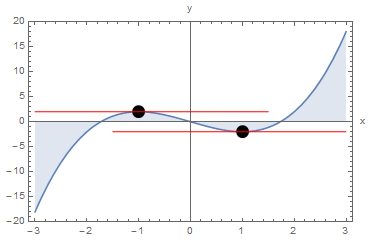
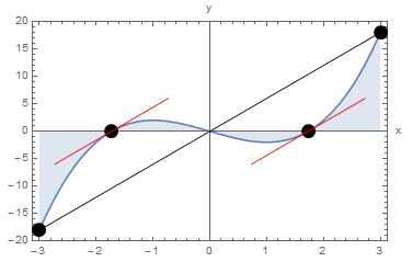
As an example, consider the function $f:[-3,3]\rightarrow \mathbb{R}$ with the relationship $f(x)=x^3-3x$ . In this case, $f(-1)=2$ is a local maximum value for $f$ attained at $x=-1$ and $f(1)=-2$ is a local minimum value of $f$ attained at $x=1$ . These local extrema values are associated with a zero slope for the function $f$ since

$f'(x)=\frac{\mathrm{d}f}{\mathrm{d}x}=3x^2-3$

$x=-1$ and $x=1$ are locations of local extrema and for both we have $f'(1)=f'(-1)=0$ . The red lines in the next figure show the slope of the function $f$ at the extremum values.

View Mathematica Code that Generated the Above Figure

Clear[x]
y = x^3 - 3 x;
Plot[y, {x, -3, 3}, Epilog -> {PointSize[0.04], Point[{-1, 2}], Point[{1, -2}], Red, Line[{{-3, 2}, {1.5, 2}}], Line[{{3, -2}, {-1.5, -2}}]}, Filling -> Axis, PlotRange -> All, Frame -> True, AxesLabel -> {"x", "y"}]

View Python Code

import numpy as np
import matplotlib.pyplot as plt
x = np.arange(-3,3,0.01)
y = x**3 - 3*x
plt.plot(x,y)
plt.fill_between(x, y, 0, alpha=0.20)
plt.plot([-3,1.5],[2,2],'r')
plt.plot([3,-1.5],[-2,-2],'r')
plt.plot([-1,1],[2,-2],'ko')
plt.xlabel('x'); plt.ylabel('y')
plt.grid(); plt.show()

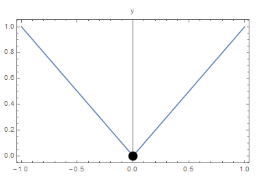
“Smoothness” or “Differentiability” is a very important requirement for the proposition to work. As an example, consider the function $f:[-1,1]\rightarrow \mathbb{R}$ defined as $f(x)=|x|$ . The function $f$ has a local minimum at $x=0$ , however, $f'(0)$ is not defined as the slope as $x\rightarrow 0$ from the right is different from the slope as $x\rightarrow 0$ from the left as shown in the next figure.

View Mathematica Code that Generated the Above Figure

Clear[x]
y = Abs[x];
Plot[y, {x, -1, 1}, Epilog -> {PointSize[0.04], Point[{0, 0}]}, PlotRange -> All, Frame -> True, AxesLabel -> {"x", "y"}]

View Python Code

import numpy as np
import matplotlib.pyplot as plt
x = np.arange(-1,1,0.01)
y = abs(x)
plt.plot(x,y)
plt.plot([0],[0],'ko')
plt.xlabel('x'); plt.ylabel('y')
plt.grid(); plt.show()

Extreme Value Theorem

Statement: Let $f:[a,b]\rightarrow \mathbb{R}$ be continuous. Then, $f$ attains its maximum and its minimum value at some points $c_{max}$ and $c_{min}$ in the interval $[a,b]$ .

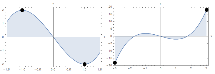
The theorem simply states that if we have a continuous function on a closed interval $[a,b]$ , then the image of $f$ contains a maximum value and a minimum value within the interval $[a,b]$ . The theorem is very intuitive. However, the proof is highly technical and relies on fundamental concepts in Real analysis including the definitions of real numbers and on continuous functions. You can review the Wikipedia entry or a course on Real analysis such as this one for details of the proof. For now, we will just illustrate the meaning of the theorem using an example. Consider the function $f:[-1.5,1.5]\rightarrow \mathbb{R}$ defined as:

$f(x)=x^3-3x$

The theorem states that $f$ has to attain a maximum value and a minimum value at a point within the interval. In this case, $f(-1)=2$ is the maximum value of $f$ attained at $x=-1\in[-1.5,1.5]$ and $f(1)=-2$ is the minimum value of $f$ attained at $x=1\in[-1.5,1.5]$ . Alternatively, if $f:[-3,3]\rightarrow \mathbb{R}$ with the same relationship as above, $f(-3)=-18$ is the minimum value of $f$ attained at $x=-3\in[-3,3]$ and $f(3)=18$ is the maximum value of $f$ attained at $x=3\in[-3,3]$
The following figure shows the graph of the function on the specified intervals.

View Mathematica Code that Generated the Above Figures

Clear[x]
y = x^3 - 3 x;
Plot[y, {x, -1.5, 1.5}, Epilog -> {PointSize[0.04], Point[{-1, 2}], Point[{1, -2}]}, Filling -> Axis, PlotRange -> All, Frame -> True, AxesLabel -> {"x", "y"}]
Plot[y, {x, -3, 3}, Epilog -> {PointSize[0.04], Point[{-3, y /. x -> -3}], Point[{3, y /. x -> 3}]}, Filling -> Axis, PlotRange -> All, Frame -> True, AxesLabel -> {"x", "y"}]

View Python Code

import numpy as np
import matplotlib.pyplot as plt
x1 = np.arange(-1.5,1.5,0.01)
y1 = x1**3 - 3*x1
plt.plot(x1,y1)
plt.fill_between(x1, y1, 0, alpha=0.20)
plt.plot([-1,1],[2,-2],'ko')
plt.xlabel('x'); plt.ylabel('y')
plt.grid(); plt.show()

x2 = np.arange(-3,3,0.01)
def f(x): return x**3 - 3*x
y2 = f(x2)
plt.plot(x2,y2)
plt.fill_between(x2, y2, 0, alpha=0.20)
plt.plot([-3,3],[f(-3),f(3)],'ko')
plt.xlabel('x'); plt.ylabel('y')
plt.grid(); plt.show()

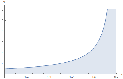
The condition that the function is defined on a closed interval $[a,b]$ is a crucial requirement for the extreme value theorem to hold true. Here is a counter example if this condition is relaxed. Let $f(x)=\frac{1}{b-x}$ defined on the open interval $(a,b)$ . The function is unbounded; it keeps increasing as $x$ approaches $b$ . The figure below provides the plot of the function $f(x)=\frac{1}{5-x}$ defined on the open interval $(4,5)$ . The function precipituously increases as it approaches the value of $f(5)$ .

Rolle’s Theorem

Statement: Let $f:[a,b]\rightarrow \mathbb{R}$ be differentiable. Assume that $f(a)=f(b)$ , then there is at least one point $c\in(a,b)$ where $f'(c)=0$ .

View Proof of Rolle's Theorem

The proof of Rolle’s theorem is straightforward from Proposition 1 and the Extreme Value Theorem above. The Extreme Value Theorem ensures that there is an extremum on the interval while Proposition 1 guarantees that the value of the first derivative is zero at the extremum point.

Let $f(a)=f(b)=g$ .

First, assume that the function is constant, i.e., $\forall x\in[a,b]: f(x)=g$ . In this case, the first derivative at every point is equal to zero. Otherwise, assume that $\exists x_0\in(a,b)$ such that $f(x_0)>g$ . The extreme value theorem asserts that $\exists x\in[a,b]$ where the function attains its extreme value, which, together with the information about $x_0$ imply that the extreme value point is an interior point to the intervial. I.e., $\exists x\in(a,b)$ where $f$ attains a maximum value. Proposition 1 then guarantees that $f'(x)=0$ . The same argument follows if $\exists x_0\in(a,b)$ such that $f(x_0)<g$ .

$\blacksquare$

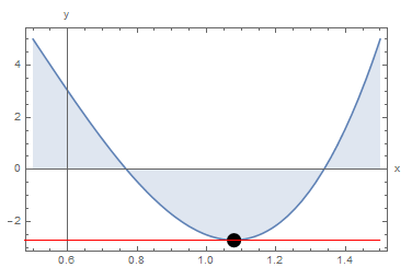
The Extreme Value Theorem ensures that there is a local maximum or local minimum within the interval, while proposition 1 ensures that at this local extremum, the slope of the function is equal to zero. As an example, consider the function $f:[0.5,1.5]\rightarrow \mathbb{R}$ defined as $f(x)=12.5-5x-30x^2+20x^3$ . $f(0.5)=f(1.5)=5$ . This ensures that there is a point $c\in(0.5,1.5)$ with $f'(c)=0$ . Indeed, $f'\left(\frac{1}{2}+\frac{1}{\sqrt{3}}\right)=0$ and the point $\frac{1}{2}+\frac{1}{\sqrt{3}}\in (0.5,1.5)$ is the location of the local minimum. The following figure shows the graph of the function on the specified interval along with the point $c$ .

View Mathematica Code that Generated the Above Figure

Clear[x]
y = 20 (x - 1/2)^3 - 20 (x - 1/2) + 5;
Expand[y]
y /. x -> 1.5
y /. x -> 0.5
y /. x -> (1/2 + 1/Sqrt[3])
D[y, x] /. x -> (1/2 + 1/Sqrt[3])
Plot[y, {x, 0.5, 1.5}, Epilog -> {PointSize[0.04], Point[{1/2 + 1/Sqrt[3], y /. x -> 1/2 + 1/Sqrt[3]}], Red, Line[{{-3, y /. x -> 1/2 + 1/Sqrt[3]}, {1.5, y /. x -> 1/2 + 1/Sqrt[3]}}]}, Filling -> Axis, PlotRange -> All, Frame -> True, AxesLabel -> {"x", "y"}]

View Python Code

import math
import numpy as np
import sympy as sp
import matplotlib.pyplot as plt

def f(x): return 20*(x - 1/2)**3 - 20*(x - 1/2) + 5
print("y(1.5):",f(1.5))
print("y(0.5):",f(0.5))
print("y(1/2 + 1/math.sqrt(3)):",f(1/2 + 1/math.sqrt(3)))
x1 = sp.symbols('x')
print("dy/dx(1/2 + 1/math.sqrt(3)):",sp.diff(20*(x1 - 1/2)**3 - 20*(x1 - 1/2) + 5,x1).subs(x1,1/2 + 1/math.sqrt(3)))

x = np.arange(0.5,1.5,0.01)
y = 20*(x - 1/2)**3 - 20*(x - 1/2) + 5
plt.plot(x,y)
plt.fill_between(x, y, 0, alpha=0.20)
plt.plot([1/2 + 1/math.sqrt(3)],[f(1/2 + 1/math.sqrt(3))],'ko')
plt.plot([0.5,1.5],[f(1/2 + 1/math.sqrt(3)),f(1/2 + 1/math.sqrt(3))],'r')
plt.xlabel('x'); plt.ylabel('y')
plt.grid(); plt.show()

Generalized Rolle’s Thoerem

Statement: Let $f:[a,b]\rightarrow \mathbb{R}$ be $n$ times differentiable. Assume that $f$ is equal to zero at $n+1$ distinct points $a< x_0<x_1<\cdots<x_n< b$ , then there is at least one point $c\in(a,b)$ where $f^{(n)}(c)=0$ .

View Proof of the Generalized Rolle's Theorem

The proof uses mathematical induction. We will first show that the argument holds for $n=1$ (2 distinct points). If $f(x_0)=f(x_1)=0$ , then, using Rolle’s theorem, $\exists \xi\in(x_0,x_1)$ such that $f'(\xi)=\frac{f(x_1)-f(x_0)}{x_1-x_0}=0$ .

Similarly, assuming that $n=2$ (three distinct points), i.e., $f(x_0)=f(x_1)=f(x_2)=0$ , then using the result from $n=1$ , $\exists \xi_1\in(x_0,x_1)$ and $\xi_2\in(x_1,x_0)$ such that $f'(\xi_1)=f'(\xi_2)=0$ . Using the results from the first case, $\exists \xi_3\in(\xi_1,\xi_2)$ such that $f''(\xi_3)=0$ .

The argument follows for higher values of $n$ leading to the statement of the theorem: if $f(x)$ has (n+1) distinct zeros $x_0<x_1<\cdots <x_n, \exists \xi\in (x_0,x_n)$ such that:

$f^{(n)}(\xi)=0$

$\blacksquare$

Mean Value Theorem

Statement: Let $f:[a,b]\rightarrow \mathbb{R}$ be differentiable. Then, there is at least one point $c\in(a,b)$ such that $f'(c)=\frac{f(b)-f(a)}{b-a}$ .

View Proof of Mean Value Theorem

The proof of the mean value theorem is straightforward by applying Rolle’s theorem to the function $g:[a,b]\rightarrow \mathbb{R}$ defined as:

$g(x)=f(x)-f(a)- \frac{f(b)-f(a)}{b-a}(x-a)$

Clearly, $g$ satisfies the conditions of Rolle’s theorem (Differentiable and $g(a)=g(b)=0$ ). We also have:

$g'(x)=f'(x)-\frac{f(b)-f(a)}{b-a}$

Therefore, by Rolle’s theorem, there is a point $c\in(a,b)$ such that $g'(c)=0\Rightarrow f'(c)=\frac{f(b)-f(a)}{b-a}$ .

$\blacksquare$

The mean value theorem states that there is a point $c$ inside the interval such that the slope of the function at $c$ is equal to the average slope along the interval. The following example will serve to illustrate the main concept of the mean value theorem. Consider the function $f:[-3,3]\rightarrow \mathbb{R}$ defined as:

$f(x)=x^3-3x$

The slope or first derivative of $f$ is given by:

$f'(x)=3x^2-3$

The average slope of $f$ on the interval is given by:

$\mbox{average slope}=\frac{f(b)-f(a)}{b-a}=\frac{f(3)-f(-3)}{3-(-3)}=\frac{2 \times 18}{6}=6$

The two points $x=\sqrt{3}$ and $x=-\sqrt{3}$ have a slope equal to the average slope:

$f'(\sqrt{3})=f'(-\sqrt{3})=3\times 3-3=6$

The figure below shows the function $f$ on the specified interval. The line representing the average slope is shown in black connecting the points $(a,f(a))$ and $(b,f(b))$ . The red lines show the slopes at the points $x=\sqrt{3}$ and $x=-\sqrt{3}$ .

View Mathematica Code that Generated the Above Figure

Clear[x]
y = x^3 - 3 x;
averageslope = ((y /. x -> 3) - (y /. x -> -3))/(3 + 3)
dydx = D[y, x];
a = Solve[D[y, x] == averageslope, x]
Point1 = {x /. a[[1, 1]], y /. a[[1, 1]]}
Point2 = {x /. a[[2, 1]], y /. a[[2, 1]]}
Plot[y, {x, -3, 3},  Epilog -> {PointSize[0.04], Point[{-3, y /. x -> -3}], Point[{3, y /. x -> 3}], Line[{{-3, y /. x -> -3}, {3, y /. x -> 3}}], Point[Point1],Point[Point2], Red, Line[{Point1 + {-1, -averageslope}, Point1, Point1 + {1, averageslope}}], Line[{Point2 + {-1, -averageslope}, Point2, Point2 + {1, averageslope}}]}, Filling -> Axis, PlotRange -> All, Frame -> True, AxesLabel -> {"x", "y"}]

View Python Code

import numpy as np
import sympy as sp
import matplotlib.pyplot as plt

def f(x): return x**3 - 3*x
averageSlope = (f(3) - f(-3))/(3 + 3)
print("averageSlope:",averageSlope)
x1 = sp.symbols('x')
dydx = sp.diff(x1**3 - 3*x1,x1)
print("dy/dx:",dydx)
sol = list(sp.solveset(dydx - averageSlope,x1))
print("Solve:",sol)

Point1 = [sol[0], f(sol[0])]
Point2 = [sol[1], f(sol[1])]
print("Point1:",Point1)
print("Point2:",Point2)

x = np.arange(-3,3,0.01)
y = x**3 - 3*x
plt.plot(x,y)
plt.fill_between(x, y, 0, alpha=0.20)
plt.plot([-3,3,Point1[0],Point2[0]],[f(-3),f(3),Point1[1],Point2[1]],'ko')
plt.plot([Point1[0]-1,Point1[0]+1,Point1[0]],
         [Point1[1]-averageSlope,Point1[1]+averageSlope,Point1[1]],'r')
plt.plot([Point2[0]-1,Point2[0]+1,Point2[0]],
         [Point2[1]-averageSlope,Point2[1]+averageSlope,Point2[1]],'r')
plt.plot([-3,3],[f(-3),f(3)],'k')
plt.xlabel('x'); plt.ylabel('y')
plt.grid(); plt.show()

First and Second Derviative Tests

The Mean Value Theorem precipitates two important results that are fundamental to analyze the behaviour of functions around their extreme values. First, we define the notion of increasing and decreasing functions

Definition: Increasing and Decreasing Functions

Let $f:(a,b)\rightarrow\mathbb{R}$ , then:

$f$ is increasing if $\forall x_1<x_2$ in $(a,b), f(x_1)\leq f(x_2)$
$f$ is decreasing if $\forall x_1<x_2$ in $(a,b), f(x_1)\geq f(x_2)$

A function is stricly increasing or decreasing if $f(x_1)< f(x_2)$ or $f(x_1)> f(x_2)$ respectively.

Proposition 2: First Derivative Test

Let $f:[a,b]\rightarrow \mathbb{R}$ be a continuous and smooth function. Then:

If $\forall x\in(a,b):f'(x)>0$ then $f$ is increasing
If $\forall x\in(a,b):f'(x)<0$ then $f$ is decreasing
If $\forall x\in(a,b):f'(x)=0$ then $f$ is constant

View Proof of the First Derivative Test

Assume $\forall x\in(a,b):f'(x)>0$ . Let $x_1<x_2$ in $(a,b)$ . Using the mean value theorem, $\exists c\in(x_1,x_2)$ such that

$f'(c)=\frac{f(x_2)-f(x_1)}{x_2-x_1}$

As $c\in(a,b)$ , therefore $f'(c)>0$ implying that $f(x_2)>f(x_1)$ . Therefore, $f$ is increasing. Similar arguments follow for the second case and third cases.

$\blacksquare$

Proposition 3: Second Derivative Test

Let $f:[a,b]\rightarrow \mathbb{R}$ be a continuous and smooth function. Let $c\in(a,b)$ be such that $f'(c)=0$ . Then:

If $f''(c)<0$ then $c$ is a local maximum
If $f''(c)>0$ then $c$ is a local minimum

View Proof of the Second Derivative Test

Since $f''(x)$ is continuous, we can assume $\exists h>0$ such that $\forall x\in (c-h,c+h):f''(x)<0$ where the interval $(c-h,c+h) \subset (a,b)$ . We will show that the function is $f$ is increasing on the interval $(c-h,c)$ and decreasing on the interval $(c,c+h)$ . Since $c$ is a local extremum by Proposition 1, therefore $c$ is a local maximum.

Let $x_1\in(c-h,c)$ . Using the mean value theorem $\exists d\in (x_1,c)$ such that:

$f''(d)=\frac{f'(c)-f'(x_1)}{c-x_1}<0$

But $f'(c)=0$ , therefore, $f'(x_1)>0$ . Since $x_1$ is arbitrary, the function is increasing on the interval $(c-h,c)$ . Similarly, let $x_1\in(c,c+h)$ . Using the mean value theorem $\exists d\in (c,x_2)$ such that:

$f''(d)=\frac{f'(x_2)-f'(c)}{x_2-c}<0$

But $f'(c)=0$ , therefore, $f'(x_2)<0$ . Since $x_2$ is arbitrary, using Proposition 2 the function is decreasing on the interval $(c,c+h)$ . I.e., the function $f$ is increasing on the left of $c$ and decreasing on the right of $c$ . Therefore, $c$ is a local maximum.

Similar arguments apply for the second case.

$\blacksquare$

This proposition is very important for optimization problems when a local maximum or minimum is to be obtained for a particular function. In order to identify whether the solution corresponds to a local maximum or minimum, the second derivative of the function can be evaluated. Considering the example given above under Proposition 1, the second derivative is given by:

$f''(x)=\frac{\mathrm{d}^2f}{\mathrm{d}x^2}=6x$

We have already identified $x=1$ and $x=-1$ as locations of the local extremum values. To know whether they are local maxima or local minima, we can evaluate the second derivative at these points. $f''(1)=6>0$ . Therefore, $x=1$ is the location of a local minimum, while $f''(-1)=-6<0$ implying that $x=-1$ is the location of a local maximum.

Taylor’s Theorem

As an introduction to Taylor’s Theorem, let’s assume that we have a function $f:\mathbb{R}\rightarrow\mathbb{R}$ that can be represented as a polynomial function in the following form:

$f(x)=b_0 + b_1 (x-a)+b_2(x-a)^2+b_3(x-a)^3+b_4(x-a)^4+\cdots + b_n(x-a)^n+\cdots$

where $a$ is a fixed point and $\forall i \geq 0: b_i$ is a constant. The best way to find these constants is to find $f$ and its derivatives when $x=a$ . So, when $x=a$ we have:

$f(a)=b_0 + b_1 (a-a)+b_2(a-a)^2+b_3(a-a)^3+b_4(a-a)^4+\cdots + b_n(a-a)^n+\cdots=b_0$

Therefore, $b_0=f(a)$ .

The derivatives of $f$ have the form:

$\begin{split}f'(x)&=b_1 +2b_2(x-a)+3b_3(x-a)^2+4b_4(x-a)^3+\cdots + nb_n(x-a)^{(n-1)}+\cdots\\f''(x)&=2b_2+2\times 3b_3(x-a)+3\times 4b_4(x-a)^2+\cdots + (n-1)nb_n(x-a)^{(n-2)}+\cdots\\\cdots\\f^{(n)}(x)&=n!b_n+\cdots\\\end{split}$

The derivatives of $f$ when $x=a$ have the form:

$\begin{split}f'(a)&=b_1 +2b_2(a-a)+3b_3(a-a)^2+4b_4(a-a)^3+\cdots + nb_n(a-a)^{(n-1)}+\cdots\\f''(a)&=2b_2+2\times 3b_3(a-a)+3\times 4b_4(a-a)^2+\cdots + (n-1)nb_n(a-a)^{(n-2)}+\cdots\\\cdots\\f^{(n)}(a)&=n!b_n+\cdots\end{split}$

Therefore, $\forall n\geq 0$ :

$b_n=\frac{f^{(n)}(a)}{n!}$

The above does not really serve as a rigorous proof for Taylor’s Theorem but rather an illustration that if an infinitely differentiable function can be represented as the sum of an infinite number of polynomial terms, then, the Taylor series form of a function defined at the beginning of this section is obtained. The following is the exact statement of Taylor’s Theorem:

Statement of Taylor’s Theorem: Let $f:\mathbb{R}\rightarrow \mathbb{R}$ be $n+1$ times differentiable on an open interval $I$ . Let $a\in I$ . Then, $\forall x \in I:\exists \xi$ between $a$ and $x$ such that:

$f(x)=f(a)+f'(a) (x-a)+\frac{f''(a)}{2!}(x-a)^2+\frac{f'''(a)}{3!}(x-a)^3+\cdots+\frac{f^{(n)}(a)}{n!}(x-a)^n+\frac{f^{(n+1)}(\xi)}{(n+1)!}(x-a)^{n+1}$

There are many proofs that can be found online for Taylor’s Theorem. Fundamentally, all of them rely on the Mean Value Theorem. We provide one proof in the expandable box below.

View Proof of Taylor's Theorem

This proof is based on this link. Fix the points $a$ and $x$ and let $t\in[a,x]$ . Define a function $G(t)$ which provides the difference between $f(x)$ and the polynomial expantion around point $t$ as follows:

$G(t)=f(x)-P_t(x)=f(x)-f(t)-f'(t)(x-t)-\frac{f''(t)}{2!}(x-t)^2-\cdots-\frac{f^{(n)}(t)}{n!}(x-t)^n$

Notice that substituting $t$ with $x$ gives:

$G(x)=f(x)-P_x(x)=f(x)-f(x)=0$

The derivative of $G$ with respect to its variable $t$ gives:

$G'(t)=-f'(t)-f''(t)(x-t)+f'(t)+\cdots-\frac{f^{(n+1)}(t)}{n!}(x-t)^n+\frac{f^{(n)}(t)}{(n-1)!}(x-t)^{n-1}=-\frac{f^{(n+1)}(t)}{n!}(x-t)^n$

Define a new function of $t$ given by:

$H(t)=G(t)-\left(\frac{x-t}{x-a}\right)^{n+1}G(a)$

The derivative of $H$ with respect to $t$ gives:

$\begin{split} H'(t)&=G'(t)+(n+1)\left(\frac{(x-t)^n}{(x-a)^{n+1}}\right)G(a)\\ &=-\frac{f^{(n+1)}(t)}{n!}(x-t)^n+(n+1)\left(\frac{(x-t)^n}{(x-a)^{n+1}}\right)G(a) \end{split}$

Evaluating the function $H$ at the points $t=x$ and $t=a$ gives:

$H(a)=0, H(x)=G(x)=0$

Using the Mean Value Theorem, $\exists \xi \in (a,x)$ such that:

$H'(\xi)=\frac{H(x)-H(a)}{x-a}=0=-\frac{f^{(n+1)}(\xi)}{n!}(x-\xi)^n+(n+1)\left(\frac{(x-\xi)^n}{(x-a)^{n+1}}\right)G(a)$

Rearranging:

$G(a)=\frac{f^{(n+1)}(\xi)}{(n+1)!}(x-a)^{n+1}$

Which is the difference between $f(x)$ and the polynomial expantion around the point $a$ .

$\blacksquare$

Explanation and Importance: Taylor’s Theorem has numerous implications in analysis in engineering. In the following we will discuss the meaning of the theorem and some of its implications:

Simply put, Taylor’s Theorem states the following: if the function $f$ and its $n+1$ derivatives are known at a point $a$ , then, the function at a point $x$ away from $a$ can be approximated by the value of the Taylor’s approximation $P_n(x)$ :

$f(x)\approx P_n(x)=f(a)+f'(a) (x-a)+\frac{f''(a)}{2!}(x-a)^2+\frac{f'''(a)}{3!}(x-a)^3+\cdots+\frac{f^{(n)}(a)}{n!}(x-a)^n$

The error (difference between the approximation $P_n(x)$ and the exact $f(x)$ is given by:

$E=f(x)-P_n(x)=\frac{f^{(n+1)}(\xi)}{(n+1)!}(x-a)^{n+1}$

The term $f^{(n+1)}(\xi)$ is bounded since $f^{(n+1)}$ is a continuous function on the interval from $a$ to $x$ . Therefore, when $x>a$ , the upper bound of the error can be given as:

$|E|\leq \max_{\xi\in[a,x]}\frac{|f^{(n+1)}(\xi)|}{(n+1)!}(x-a)^{n+1}$

While, when $x<a$ , the upper bound of the error can be given as:

$|E|\leq \max_{\xi\in[x,a]}\frac{|f^{(n+1)}(\xi)|}{(n+1)!}(a-x)^{n+1}$

The above implies that the error is directly proportional to $(x-a)^{n+1}$ . This is traditionally written as follows:
$f(x)=P_n(x)+\mathcal{O} (h^{n+1})$

where $h=(x-a)$ . In other words, as $x-a$ gets smaller and smaller, the error gets smaller in proportion to $(x-a)^{n+1}$ . As an example, if we choose $x_1-a=0.1$ and then $x_2-a=0.05$ , then, $\frac{E_1}{E_2}\geq\left(\frac{0.1}{0.05}\right)^{n+1}=2^{n+1}$ . I.e., if the step size is halved, the error is divided by $2^{n+1}$ .
If the function $f:[c,d]\rightarrow \mathbb{R}$ is infinitely differentiable on an interval $I$ , and if $a\in I$ , then $\forall x\in I:f(x)$ is the limit of the sum of the Taylor series. The error which is the difference between the infinite sum and the approximation is called the truncation error as defined in the error section.
There are many rigorous proofs available for Taylor’s Theorem and the majority rely on the mean value theorem above. Notice that if we choose $n=0$ , then the mean value theorem is obtained. For a rigorous proof, you can check one of these links: link 1 or link 2. Note that these proofs rely on the mean value theorem. In particular, L’Hôpital’s rule was used in the Wikipedia proof which in turn relies on the mean value theorem.

The following code illustrates the difference between the function $f(x)=\sin{x}+0.01x^2$ and the Taylor’s polynomial $P(x)$ . You can download the code, change the function, the point $a$ , and the range of the plot to see how the Taylor series of other functions behave.

View Mathematica Code

Taylor[y_, x_, a_, n_] := (y /. x -> a) + 
  Sum[(D[y, {x, i}] /. x -> a)/i!*(x - a)^i, {i, 1, n}]
f = Sin[x] + 0.01 x^2;
Manipulate[
 s = Taylor[f, x, 1, nn];
 Grid[{{Plot[{f, s}, {x, -10, 10}, PlotLabel -> "f(x)=Sin[x]+0.01x^2",
      PlotLegends -> {"f(x)", "P(x)"}, 
     PlotRange -> {{-10, 10}, {-6, 30}}, 
     ImageSize -> Medium]}, {Expand[s]}}], {nn, 1, 30, 1}]

View Python Code

import math
import numpy as np
import sympy as sp
import matplotlib.pyplot as plt
from ipywidgets.widgets import interact

def taylor(f,xi,a,n):
  return sum([(f.diff(x1,i).subs(x1,a))/math.factorial(i)*(xi - a)**i for i in range(n)])

x1 = sp.symbols('x')
f = sp.sin(x1) + 0.01*x1**2

@interact(n=(1,30,1))
def update(n=1):
  x = np.arange(-10,10,0.1)
  y = np.sin(x) + 0.01*x**2
  plt.plot(x,y, label="f(x)")
  
  p = [taylor(f,xi,1,n) for xi in x]
  plt.plot(x,p, label="P(x)")
  plt.title("")
  plt.xlabel('x'); plt.ylabel('y')
  plt.ylim(-6,30); plt.xlim(-10,10)
  plt.legend(); plt.grid(); plt.show()
  print(sp.series(f,x1,0,n))

The following tool illustrates the difference between the function $f(x)=\sin{x}+0.01x^2$ and the Taylor’s polynomial $P(x)$ . You can change the order of the series expansion to see how the Taylor series of the function behave.

The Mathematica function Series can also be used to generate the Taylor expansion of any function:

View Mathematica Code

Series[Tan[x],{x,0,7}]
Series[1/(1+x^2),{x,0,10}]

View Python Code

import sympy as sp
sp.init_printing(use_latex=True)
x = sp.symbols('x')
display("tan(x):",sp.series(sp.tan(x),x,0,8))
display("1/(1+x**2):",sp.series(1/(1+x**2),x,0,11))

The following tool shows how the Taylor series expansion around the point $a=1$ , termed $P(x)$ in the figure, can be used to provide an approximation of different orders to a cubic polynomial, termed $f(x)$ in the figure. Use the buttons to change the order of the series expansion. The tool provides the error at $x=3$ , namely $E=f(3)-P(3)$ . What happens when the order reaches 3?

Polynomial Interpolation Error

While not related to the Taylor’s Theorem, the error in the interpolating polynomial can be shown to have a form similar to the Taylor’s Theorem error term. The following theorem will be used later in the book when evaluating the error associated with the interpolating polynomial. Similar to Taylor’s Theorem, the proof relies on the Mean Value Theorem above.

Statement of Polynomial Interpolation Error Theorem: Let $f:\mathbb{R}\rightarrow \mathbb{R}$ be $n+1$ times differentiable on an open interval $I=(x_0,x_n)$ . Let $x_0<x_1<x_2<x_3<\cdots<x_n$ and define the $n$ degree interpolating polynomial

$p(x)=A_0+A_1(x-x_0)+A_2(x-x_0)(x-x_1)+\cdots+A_n(x-x_0)\cdots (x-x_{n-1})$

Then, $\forall x \in I:\exists \xi$ between $x_0$ and $x_n$ such that:

$f(x)-p(x)=\frac{f^{(n+1)}(\xi)}{(n+1)!}\prod_{i=0}^n(x-x_i)$

View Proof of Polynomial Interpolation Error Theorem

This proof is based on this link. Another useful link which provides some intuitive relation between the Polynomial Interpolation Error and the Taylor Theorem can be found here.

The error between the interpolating polynomial and the function can be defined as:

$E(x)=f(x)-p(x)$

Notice that $E(x_0)=E(x_1)=\cdots=E(x_n)=0$ as the interpolating polynomial coefficients $A_i$ are obtained by solving the $n+1$ equations of the form $f(x_i)=p(x_i)$ where $0\leq i \leq n$ . Fix $x\in (x_0,x_n)$ such that $\forall i,x\neq x_i$ and define the function $K(t)$ as:

$K(t)=E(t)-E(x)\frac{W(t)}{W(x)}$

Where

$W(x)=\prod_{i=0}^n(x-x_i)$

Utilizing the fact that $p^{(n+1)}(t)=0$ , the $n+1$ derivative of $K$ is given by:

$K^{(n+1)}(t)=f^{(n+1)}(t)-E(x)\frac{(n+1)!}{W(x)}$

Notice that $\forall i:K(x_i)=E(x_i)-E(x)\frac{W(x_i)}{W(x)}=0$ and $K(x)= 0$ . I.e., $K(t)$ has $n+2$ distinct roots. Using the generalized Rolle’s theorem, $\exists \xi\in[x_0,x_n]$ such that $K^{(n+1)}(\xi)=0$ . Therefore:

$E(x)=f^{(n+1)}(\xi)\frac{W(x)}{(n+1)!}$

$\blacksquare$

Page Comments

Jaskaran Pandher says:

March 11, 2024 at 7:21 pm

This was expertly explained. I know this is a conceptual topic that requires focus and clear definition. I appreciated this resource a lot.

Reply
1. Samer Adeeb says:
  
  March 11, 2024 at 9:27 pm
  
  Thank you!
  
  Reply

Open Educational Resources

Taylor Series: Mathematical Background

Definitions

Taylor’s Theorem

Extreme Values of Smooth Functions

Definition: Local Maximum and Local Minimum

Proposition 1

Extreme Value Theorem

Rolle’s Theorem

Generalized Rolle’s Thoerem

Mean Value Theorem

First and Second Derviative Tests

Definition: Increasing and Decreasing Functions

Proposition 2: First Derivative Test

Proposition 3: Second Derivative Test

Taylor’s Theorem

Polynomial Interpolation Error

Page Comments

Leave a Reply Cancel reply