Engineering at Alberta Courses » Runge-Kutta Methods

Solution Methods for IVPs: Runge-Kutta Methods

Runge-Kutta Methods

The Runge-Kutta methods developed by the German mathematicians C. Runge and M.W. Kutta are essentially a generalization of all the previous methods. Consider the following IVP:

$\frac{\mathrm{d}x}{\mathrm{d}t}=F(x,t)$

Assuming that the value of the dependent variable $x$ (say $x_i$ ) is known at an initial value $t_i$ , then, the Runge-Kutta methods employ the following general equation to calculate the value of $x$ at $t=t_{i+1}$ , namely $x_{i+1}$ with $h=t_{i+1}-t_i$ :

$x_{i+1}=x_i+h\phi$

where $\phi$ is a function of the form:

$\phi=\alpha_1 k_1+\alpha_2k_2+\alpha_3k_3+\cdots+\alpha_nk_n$

$\alpha_j$ are constants while $k_j=F(x,t)$ evaluated at points within the interval $[x_i,x_{i+1}]$ and have the form:

$\begin{split}k_1&=F(x_i,t_i)\\k_2&=F(x_i+q_{11}k_1h,t_i+p_1h)\\k_3&=F(x_i+q_{21}k_1h+q_{22}k_2h,t_i+p_2h)\\&\vdots\\k_n&=F(x_i+q_{(n-1),1}k_1h+q_{(n-1),2}k_2h+\cdots+q_{(n-1),(n-1)}k_{n-1}h,t_i+p_{n-1}h)\end{split}$

The constants $\alpha_j$ , and the forms of $k_j$ are obtained by equating the value of $x_{i+1}$ obtained using the Runge-Kutta equation to a particular form of the Taylor series. The $k's$ are recurrence relationships, meaning $k_1$ appears in $k_2$ , which appears in $k_3$ , and so forth. This makes the method efficient for computer calculations. The error in a particular form depends on how many terms are used. The general forms of these Runge-Kutta methods could be implicit or explicit. For example, the explicit Euler method is a Runge-Kutta method with only one term with $\alpha_1=1$ and $k_1=F(x_i,t_i)$ . Heun’s method on the other hand is a Runge-Kutta method with the following non-zero terms:

$\begin{split}\alpha_1&=\alpha_2=\frac{1}{2}\\k_1&=F(x_i,t_i)\\k_2&=F(x_i+hk_1,t_i+h)\end{split}$

Similarly, the midpoint method is a Runge-Kutta method with the following non-zero terms:

$\begin{split}\alpha_2&=1\\k_1&=F(x_i,t_i)\\k_2&=F(x_i+\frac{h}{2}k_1,t_i+\frac{h}{2})\end{split}$

The most popular Runge-Kutta method is referred to as the “classical Runge-Kutta method”, or the “fourth-order Runge-Kutta method”. It has the following form:

$x_{i+1}=x_i+\frac{h}{6}\left(k_1+2k_2+2k_3+k_4\right)$

with

$\begin{split}k_1&=F(x_i,t_i)\\k_2&=F\left(x_i+\frac{h}{2}k_1,t_i+\frac{h}{2}\right)\\k_3&=F\left(x_i+\frac{h}{2}k_2,t_i+\frac{h}{2}\right)\\k_4&=F(x_i+hk_3,t_i+h)\end{split}$

The error in the fourth-order Runge-Kutta method is similar to that of the Simpson’s 1/3 rule, with a local error term $E_{\mbox{local}}=\mathcal{O}(h^5)$ which would translate into a global error term of $E=\mathcal{O}(h^4)$ . The method is termed fourth-order because the error term is directly proportional to the step size raised to the power of 4.

View Mathematica Code

RK4Method[fp_, x0_, h_, t0_, tmax_] := (n = (tmax - t0)/h + 1;
  xtable = Table[0, {i, 1, n}];
  xtable[[1]] = x0;
  Do[k1 = fp[xtable[[i - 1]], t0 + (i - 2) h];
   k2 = fp[xtable[[i - 1]] + h/2*k1, t0 + (i - 1.5) h];
   k3 = fp[xtable[[i - 1]] + h/2*k2, t0 + (i - 1.5) h];
   k4 = fp[xtable[[i - 1]] + h*k3, t0 + (i - 1) h];
   xtable[[i]] = xtable[[i - 1]] + h (k1 + 2 k2 + 2 k3 + k4)/6, {i, 2,
     n}];
  Data2 = Table[{t0 + (i - 1)*h, xtable[[i]]}, {i, 1, n}];
  Data2)

View Python Code

def RK4Method(fp, x0, h, t0, tmax):
  n = int((tmax - t0)/h + 1)
  xtable = [0 for i in range(n)]
  xtable[0] = x0
  for i in range(1,n):
    k1 = fp(xtable[i - 1], t0 + (i - 1)*h)
    k2 = fp(xtable[i - 1] + h/2*k1, t0 + (i - 0.5)*h)
    k3 = fp(xtable[i - 1] + h/2*k2, t0 + (i - 0.5)*h)
    k4 = fp(xtable[i - 1] + h*k3, t0 + i*h)
    xtable[i] = xtable[i - 1] + h*(k1 + 2*k2 + 2*k3 + k4)/6 
  Data = [[t0 + i*h, xtable[i]] for i in range(n)]
  return Data

Example

Solve Example 4 above using the classical Runge-Kutta method but with $h=0.4$ .

Solution

Recall the differential equation of this problem:

$\frac{\mathrm{d}x}{\mathrm{d}t}=F(x,t)=tx^2+2x$

Setting $x_0=-5$ , $t_0=0$ , $h=0.4$ , the following are the values of $k_1$ , $k_2$ , $k_3$ , and $k_4$ required to calculate $x_1$ :

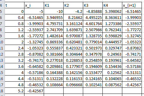
$\begin{split}k_1&=F(x_0,t_0)=F(-5,0)\\&=0+2(-5)=-10\\k_2&=F\left(x_0+\frac{h}{2}k_1,t_0+\frac{h}{2}\right)=F(-5+0.2(-10),0+0.2)\\&=0.2(-5+0.2(-10))^2+2\times (-5+0.2(-10))=-4.2\\k_3&=F\left(x_0+\frac{h}{2}k_2,t_0+\frac{h}{2}\right)=F(-5+0.2(-4.2),0+0.2)\\&=0.2(-5+0.2(-4.2))^2+2\times (-5+0.2(-4.2))=-4.8589\\k_4&=F(x_0+hk_3,t_0+h)=F(-5+0.4(-4.8589),0+0.4)\\&=0.4(-5+0.4(-4.8589))^2+2\times(-5+0.4(-4.8589))=5.3981\end{split}$

Therefore:

$x_1=x_0+\frac{h}{6}(k_1+2k_2+2k_3+k_4)=-5+\frac{0.4}{6}(-10-2\times 4.2-2\times 4.8589+5.3981)=-6.51465$

Proceeding iteratively gives the values of $x_i$ up to $t=5.2$ . The Microsoft Excel file RK4.xlsx provides the required calculations. The following Microsoft Excel table shows the required calculations:

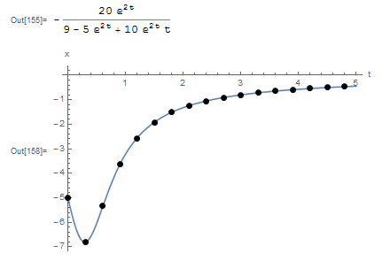
The following Mathematica code implements the classical Runge-Kutta method for this problem with $h=0.3$ . The output curve is shown underneath.

View Mathematica Code

RK4Method[fp_, x0_, h_, t0_, tmax_] := (n = (tmax - t0)/h + 1;
  xtable = Table[0, {i, 1, n}];
  xtable[[1]] = x0;
  Do[k1 = fp[xtable[[i - 1]], t0 + (i - 2) h];
   k2 = fp[xtable[[i - 1]] + h/2*k1, t0 + (i - 1.5) h];
   k3 = fp[xtable[[i - 1]] + h/2*k2, t0 + (i - 1.5) h];
   k4 = fp[xtable[[i - 1]] + h*k3, t0 + (i - 1) h];
   xtable[[i]] = xtable[[i - 1]] + h (k1 + 2 k2 + 2 k3 + k4)/6, {i, 2,
     n}];
  Data2 = Table[{t0 + (i - 1)*h, xtable[[i]]}, {i, 1, n}];
  Data2)
Clear[x, xtable]
a = DSolve[{x'[t] == t*x[t]^2 + 2*x[t], x[0] == -5}, x, t];
x = x[t] /. a[[1]]
fp[x_, t_] := t*x^2 + 2*x;
Data2 = RK4Method[fp, -5.0, 0.3, 0, 5];
Plot[x, {t, 0, 5}, Epilog -> {PointSize[Large], Point[Data2]},  AxesOrigin -> {0, 0}, AxesLabel -> {"t", "x"}, PlotRange -> All]
Title = {"t_i", "x_i"};
Data2 = Prepend[Data2, Title];
Data2 // MatrixForm

View Python Code

# UPGRADE: need Sympy 1.2 or later, upgrade by running: "!pip install sympy --upgrade" in a code cell
# !pip install sympy --upgrade
import numpy as np
import sympy as sp
import matplotlib.pyplot as plt
sp.init_printing(use_latex=True)

def RK4Method(fp, x0, h, t0, tmax):
  n = int((tmax - t0)/h + 1)
  xtable = [0 for i in range(n)]
  xtable[0] = x0
  for i in range(1,n):
    k1 = fp(xtable[i - 1], t0 + (i - 1)*h)
    k2 = fp(xtable[i - 1] + h/2*k1, t0 + (i - 0.5)*h)
    k3 = fp(xtable[i - 1] + h/2*k2, t0 + (i - 0.5)*h)
    k4 = fp(xtable[i - 1] + h*k3, t0 + i*h)
    xtable[i] = xtable[i - 1] + h*(k1 + 2*k2 + 2*k3 + k4)/6 
  Data = [[t0 + i*h, xtable[i]] for i in range(n)]
  return Data

x = sp.Function('x')
t = sp.symbols('t')
sol = sp.dsolve(x(t).diff(t) - t*x(t)**2 - 2*x(t), ics={x(0): -5})
display(sol)
def fp(x, t): return t*x**2 + 2*x
Data = RK4Method(fp, -5.0, 0.3, 0, 5)
x_val = np.arange(0,5,0.01)
plt.plot(x_val, [sol.subs(t, i).rhs for i in x_val])
plt.scatter([point[0] for point in Data],[point[1] for point in Data],c='k')
plt.xlabel("t"); plt.ylabel("x")
plt.grid(); plt.show()
print(["t_i", "x_i"],"\n",np.vstack(Data))

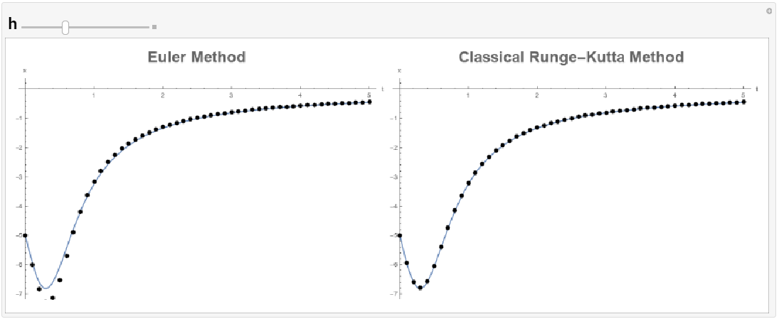
MATLAB files: File 1 (ex12_10.m) File 2 (rk4.m)

The following tool provides a comparison between the explicit Euler method and the classical Runge-Kutta method. The classical Runge-Kutta method gives excellent predictions even when $h=0.5$ , at which point the explicit Euler method fails to predict anything close to the exact equation. The classical Runge-Kutta method also provides better estimates than the midpoint method and Heun’s method above.

Open Educational Resources

Solution Methods for IVPs: Runge-Kutta Methods

Runge-Kutta Methods

Example

Solution

Lecture Video

Leave a Reply Cancel reply