
Numerical Integration: Rectangle Method
Rectangle Method
Let ![f:[a,b]\rightarrow \mathbb{R}](https://engcourses-uofa.ca/wp-content/ql-cache/quicklatex.com-602dc0a5221796cd029651364476c9ef_l3.png "Rendered by QuickLaTeX.com") . The rectangle method utilizes the Riemann integral definition to calculate an approximate estimate for the area under the curve by drawing many rectangles with very small width adjacent to each other between the graph of the function
. The rectangle method utilizes the Riemann integral definition to calculate an approximate estimate for the area under the curve by drawing many rectangles with very small width adjacent to each other between the graph of the function  and the
  axis. For simplicity, the width of the rectangles is chosen to be constant. Let
  be the number of intervals with
  and constant spacing
  . The rectangle method can be implemented in one of the following three ways:
![\[\begin{split}I_1&=\int_{a}^b\!f(x)\,\mathrm{d}x\approx h\sum_{i=1}^{n}f(x_{i-1})\\I_2&=\int_{a}^b\!f(x)\,\mathrm{d}x\approx h\sum_{i=1}^{n}f\left(\frac{x_{i-1}+x_{i}}{2}\right)\\I_3&=\int_{a}^b\!f(x)\,\mathrm{d}x\approx h\sum_{i=1}^{n}f(x_{i})\end{split}\]](https://engcourses-uofa.ca/wp-content/ql-cache/quicklatex.com-3fd08e94cb1601a88b84012092c88aca_l3.png "Rendered by QuickLaTeX.com")
If  and
and  are the left and right points defining the rectangle number
  , then
  assumes that the height of the rectangle is equal to
  ,
,  assumes that the height of the rectangle is equal to
  , and
, and  assumes that the height of the rectangle is equal to
  . is called the midpoint rule.
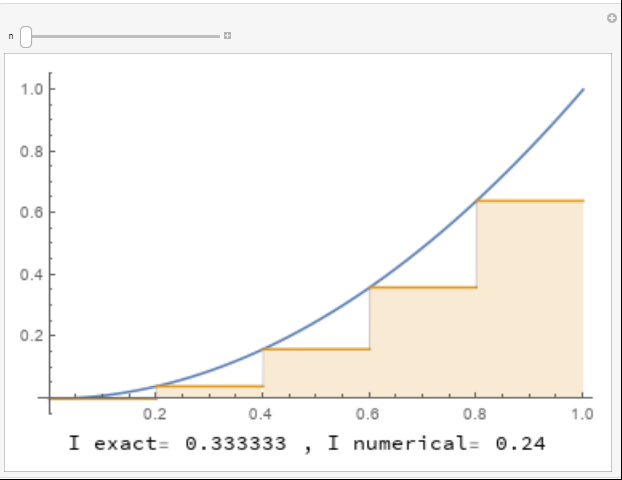
To illustrate the difference, consider the function  on the interval
 ![[0,1]](https://engcourses-uofa.ca/wp-content/ql-cache/quicklatex.com-a8b36d8d3c0436b5a9c763cbff76f47a_l3.png "Rendered by QuickLaTeX.com") . The exact integral can be calculated as
. The exact integral can be calculated as
![\[I_{\mbox{exact}}=\frac{x^3}{3}\bigg|_{x=0}^{x=1}=0.3333\]](https://engcourses-uofa.ca/wp-content/ql-cache/quicklatex.com-346020a36434e59855da27777352dba4_l3.png "Rendered by QuickLaTeX.com")
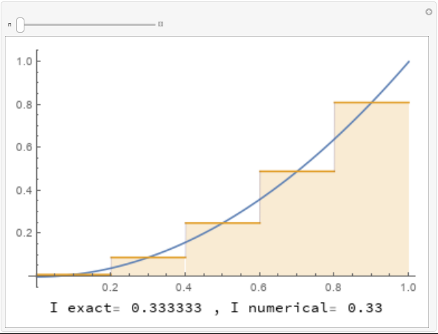
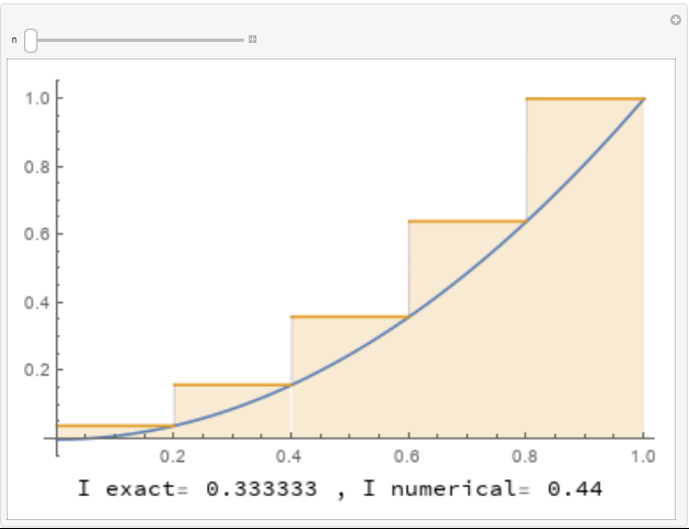
The following three tools show the implementation of the rectangle method for numerically integrating the function using , , and , respectively. For , each rectangle touches the graph of the function at the top left corner of the rectangle. For , each rectangle touches the graph of the function at the mid point of the top side. For , each rectangle touches the graph of the function at the top right corner of the rectangle. The areas of the rectangles are calculated underneath each curve. Use the slider to increase the number of rectangles to see how many rectangles are needed to get a good approximation for the area under the curve.
The following Mathematica code can be used to numerically integrate any function on the interval ![[a,b]](https://engcourses-uofa.ca/wp-content/ql-cache/quicklatex.com-1f90ba537767823131bb8d396cdc5a9c_l3.png "Rendered by QuickLaTeX.com") using the three options for the rectangle method.
using the three options for the rectangle method.
I1[f_, a_, b_, n_] := (h = (b - a)/n; Sum[f[a + (i - 1)*h]*h, {i, 1, n}])
I2[f_, a_, b_, n_] := (h = (b - a)/n; Sum[f[a + (i - 1/2)*h]*h, {i, 1, n}])
I3[f_, a_, b_, n_] := (h = (b - a)/n; Sum[f[a + (i)*h]*h, {i, 1, n}])
f[x_] := x^2;
I1[f, 0, 1, 13.0]
I2[f, 0, 1, 13.0]
I3[f, 0, 1, 13.0]
def I1(f, a, b, n):
  h = (b - a)/n
  return sum([f(a + i*h)*h for i in range(int(n))])
def I2(f, a, b, n):
  h = (b - a)/n
  return sum([f(a + (i + 1/2)*h)*h for i in range(int(n))])
def I3(f, a, b, n):
  h = (b - a)/n
  return sum([f(a + (i + 1)*h)*h for i in range(int(n))])
def f(x): return x**2
print("I1:",I1(f, 0, 1, 13.0))
print("I2:",I2(f, 0, 1, 13.0))
print("I3:",I3(f, 0, 1, 13.0))
The following link provides the MATLAB codes for implementing the rectangle method.
Error Analysis
Taylor’s theorem can be used to find how the error changes as the step size  decreases. First, let’s consider (the same applies to ). The error in the calculation of rectangle number between the points and will be estimated. Using Taylor’s theorem,
 ![\forall x\in[x_{i-1},x_{i}], \exists \xi\in[x_{i-1},x]](https://engcourses-uofa.ca/wp-content/ql-cache/quicklatex.com-fe93a07818df72a11422b1855cdcdef9_l3.png "Rendered by QuickLaTeX.com") such that:
such that:
![\[f(x)=f(x_{i-1})+f'(\xi)(x-x_{i-1})\]](https://engcourses-uofa.ca/wp-content/ql-cache/quicklatex.com-376d892b161d28e6ad8f74afd658532b_l3.png "Rendered by QuickLaTeX.com")
The error in the integral using this rectangle can be calculated as follows:
![\[\begin{split}|E_i|&=\left|\int_{x_{i-1}}^{x_{i}}\!f(x)-f(x_{i-1})\,\mathrm{d}x\right|=\left|\int_{x_{i-1}}^{x_{i}}\!f'(\xi)(x-x_{i-1})\,\mathrm{d}x\right|\\&\leq \max_{\xi\in[x_{i-1},x_i]}|f'(\xi)|\frac{(x-x_{i-1})^2}{2}\bigg|_{x_{i-1}}^{x_i}=\max_{\xi\in[x_{i-1},x_i]}|f'(\xi)|\frac{h^2}{2}\end{split}\]](https://engcourses-uofa.ca/wp-content/ql-cache/quicklatex.com-1e9f515fc1d504fcbbcf316baa5a90de_l3.png "Rendered by QuickLaTeX.com")
If is the number of subdivisions (number of rectangles), i.e.,  , then:
![\[|E|=|nE_i| \leq \max_{\xi\in[a,b]}|f'(\xi)| n\frac{h^2}{2}=\max_{\xi\in[a,b]}|f'(\xi)| (b-a)\frac{h}{2}\]](https://engcourses-uofa.ca/wp-content/ql-cache/quicklatex.com-a5c11f4a509a63be159497c3c5b424f0_l3.png "Rendered by QuickLaTeX.com")
In other words, the total error is bounded by a term that is directly proportional to . When decreases, the error bound decreases proportionally. Of course when goes to zero, the error goes to zero as well.
(Midpoint rule) provides a faster convergence rate, or a more accurate approximation as the error is bounded by a term that is directly proportional to  as will be shown here.
Using Taylor’s theorem, such that:
![\[f(x)=f(x_{m})+f'(x_i)(x-x_{m})+f''(\xi)\frac{(x-x_{m})^2}{2}\]](https://engcourses-uofa.ca/wp-content/ql-cache/quicklatex.com-d2f90d4aec48f5073bec5aae5e619959_l3.png "Rendered by QuickLaTeX.com")
Where  . The error in the integral using this rectangle can be calculated as follows:
![\[\begin{split}|E_i|&=\left|\int_{x_{i-1}}^{x_{i}}\!f(x)-f(x_m)\,\mathrm{d}x\right|=\left|f'(x_i)\int_{x_{i-1}}^{x_{i}}\!(x-x_m)\,\mathrm{d}x+\int_{x_{i-1}}^{x_{i}}\!\frac{f''(\xi)}{2}(x-x_m)^2\,\mathrm{d}x\right|\\&=\left|f'(x_i)\frac{(x_i-x_m)^2-(x_{i-1}-x_m)^2}{2}+\int_{x_{i-1}}^{x_{i}}\!\frac{f''(\xi)}{2}(x-x_m)^2\,\mathrm{d}x\right|\\&=\left|0+\int_{x_{i-1}}^{x_{i}}\!\frac{f''(\xi)}{2}(x-x_m)^2\,\mathrm{d}x\right|\\&\leq \max_{\xi\in[x_{i-1},x_i]}\frac{|f''(\xi)|}{2}\frac{\left(\frac{h}{2}\right)^3-\left(\frac{-h}{2}\right)^3}{3}\\&\leq \max_{\xi\in[x_{i-1},x_i]}\frac{|f''(\xi)|}{24}h^3\end{split}\]](https://engcourses-uofa.ca/wp-content/ql-cache/quicklatex.com-e4e69a65859e338cd805fbb84df58fbe_l3.png "Rendered by QuickLaTeX.com")
If is the number of subdivisions (number of rectangles), i.e., , then:
![\[|E|=|nE_i| \leq \max_{\xi\in[a,b]}|f''(\xi)| n\frac{h^3}{24}=\max_{\xi\in[a,b]}|f''(\xi)| (b-a)\frac{h^2}{24}\]](https://engcourses-uofa.ca/wp-content/ql-cache/quicklatex.com-34ee4e5ad9bd520c934f473a406447f1_l3.png "Rendered by QuickLaTeX.com")
In other words, the total error is bounded by a term that is directly proportional to which provides faster convergence than . The tools shown above can provide a good illustration of this. With only five rectangles, already provides a very good estimate for the integral compared to both , and .
Example
Using the rectangle method with  , calculate , , and and compare with the exact integral of the function
  on the interval
 ![[0,2]](https://engcourses-uofa.ca/wp-content/ql-cache/quicklatex.com-9ec15e699e72ba501abfc77baca9b5a6_l3.png "Rendered by QuickLaTeX.com") . Then, find the values of required so that the total error obtained by and that obtained by are bounded by 0.001.
. Then, find the values of required so that the total error obtained by and that obtained by are bounded by 0.001.
Solution
Since the spacing can be calculated as:
![\[h=\frac{b-a}{n}=\frac{2-0}{4}=0.5\]](https://engcourses-uofa.ca/wp-content/ql-cache/quicklatex.com-100f6cd89fddd893d18b00ee5caf512d_l3.png "Rendered by QuickLaTeX.com")
Therefore,  ,
,  ,
,  ,
,  , and
, and  . The values of the function at these points are given by:
![\[f(x_0)=e^0=1.00\qquad f(x_1)=e^{0.5}=1.6487 \qquad f(x_2)=e^{1}=2.7183\]](https://engcourses-uofa.ca/wp-content/ql-cache/quicklatex.com-d97c5ed315dd5b14f51ff225cd90e23d_l3.png "Rendered by QuickLaTeX.com")
![\[f(x_3)=e^{1.5}=4.4817 \qquad f(x_4)=e^{2}=7.3891\]](https://engcourses-uofa.ca/wp-content/ql-cache/quicklatex.com-5a483416a61d816f7cf5f2341555e772_l3.png "Rendered by QuickLaTeX.com")
According to the rectangle method we have:
![\[\begin{split}I_1&=\sum_{i=1}^{n}f(x_{i-1})h=0.5 (1 + 1.6487 + 2.7183 + 4.4817) = 4.924\\I_3&=\sum_{i=1}^{n}f(x_{i})h=0.5 (1.6487 + 2.7183 + 4.4817+7.3891) = 8.119\end{split}\]](https://engcourses-uofa.ca/wp-content/ql-cache/quicklatex.com-09fa2e3d16ebe96483ae9fb6c78f62d1_l3.png "Rendered by QuickLaTeX.com")
For , we need to calculate the values of the function at the midpoint of each rectangle:
![\[f\left(\frac{x_0+x_1}{2}\right)=e^{0.25}=1.284 \qquad f\left(\frac{x_1+x_2}{2}\right)=e^{0.75}=2.117\]](https://engcourses-uofa.ca/wp-content/ql-cache/quicklatex.com-02665c8786e7ad45908a47e8107ac4bf_l3.png "Rendered by QuickLaTeX.com")
![\[f\left(\frac{x_2+x_3}{2}\right)=e^{1.25}=3.49 \qquad f\left(\frac{x_3+x_4}{2}\right)=e^{1.75}=5.755\]](https://engcourses-uofa.ca/wp-content/ql-cache/quicklatex.com-9dfdb9d7bd7ea82c8ae18c1a3dd6638a_l3.png "Rendered by QuickLaTeX.com")
Therefore:
![\[I_2=\sum_{i=1}^{n}f\left(\frac{x_{i-1}+x_{i}}{2}\right)h=0.5(1.284+2.117+3.49+5.755)=6.323\]](https://engcourses-uofa.ca/wp-content/ql-cache/quicklatex.com-4986d373b4f3b7f07c5170d08dc1b4d0_l3.png "Rendered by QuickLaTeX.com")
The exact integral is given by:
![\[I=\int_{0}^2\!e^x\,\mathrm{d}x=e^2-e^0=6.38906\]](https://engcourses-uofa.ca/wp-content/ql-cache/quicklatex.com-b4e8b0f7b03c858acc2616265551a960_l3.png "Rendered by QuickLaTeX.com")
Obviously,
provides a good approximation with only 4 rectangles!
Error Bounds
The total errors obtained when  are indeed less than the error bounds obtained by the formulas listed above. For and , the error in the estimation is bounded by:
![\[|E|\leq \max_{\xi\in[a,b]}|f'(\xi)| (b-a)\frac{h}{2}=e^{2}(2-0)\frac{0.5}{2}=3.695\]](https://engcourses-uofa.ca/wp-content/ql-cache/quicklatex.com-9b573bf5509f9d0b07c08f68505cfd21_l3.png "Rendered by QuickLaTeX.com")
The errors  and
and  are indeed less than that upper bound. The same formula can be used to find the value of so that the error is bounded by 0.001:
![\[e^{2}(2-0)\frac{h}{2}=0.001\Rightarrow h=0.000135\]](https://engcourses-uofa.ca/wp-content/ql-cache/quicklatex.com-6f40778fc7d411ca5504b093b153fed5_l3.png "Rendered by QuickLaTeX.com")
Therefore, to guarantee an error less than 0.001 using , the interval will have to be divided into:  rectangles! In this case
  and
and 
Similarly, when the error in the estimate using is bounded by:
![\[|E|=\max_{\xi\in[a,b]}|f''(\xi)| (b-a)\frac{h^2}{24}=e^2(2-0)\frac{0.5^2}{24}=0.1539\]](https://engcourses-uofa.ca/wp-content/ql-cache/quicklatex.com-4532dfe097c1757d627df2b598357a22_l3.png "Rendered by QuickLaTeX.com")
The error  is indeed bounded by that upper error. The same formula can be used to find the value of so that the error is bounded by 0.001:
![\[e^2(2-0)\frac{h^2}{24}=0.001\Rightarrow h = 0.04\]](https://engcourses-uofa.ca/wp-content/ql-cache/quicklatex.com-e5f38c5d74db657fbcca43ad42db5ad0_l3.png "Rendered by QuickLaTeX.com")
Therefore, to guarantee an error less than 0.001 using , the interval will have to be divided into:  rectangles! In this case
  and
and 
Thank you for uploading informative lectures.
I have a question about error analysis for I2 (midpoint rule).
In this lecture, using Taylor’s theorem, we expand up to three terms (including the remainder term) for I2 while up to two terms for I1 (and I3). Is there a specific reason for this?
(I guess it is because we use two points, x(i-1) and x(i), to calculate the midpoint, but still this does not sound plausible to me.)
I would appreciate it if you could explain this for me.
Again, thank you for uploading your wonderful lectures.
Indeed, intuitively speaking, using the mid-point leads to a decrease in the associated error since there is tendency for positive and negative errors to cancel each other.
When attempting to find a rigorous upper bound for the error, one starts with the Taylor approximation with as many terms as possible. For the I1 and I3, having more than two terms will not enable finding an upper bound. For I2, with three terms, it is possible to find an upper bound as per the derivation above.
Thank you for your explanation. Now I can see it.
I have a small doubt….
For the case of Midpoint formula, the Taylor series expansion is written as f(x) = f(xm) + f'(xi)*(x-xm) + f”(e)*((x-xm)^2)/2.
Can we write the Taylor series as: f(x) = f(xm) + f'(xm)*(x-xm) + f”(e)*((x-xm)^2)/2. ?????
(notice the difference in the coeffiecient of (x-xm)