
Nonlinear Systems of Equations: Linear vs. Nonlinear Analysis
Linear vs. Nonlinear Analysis of Structures: An Application
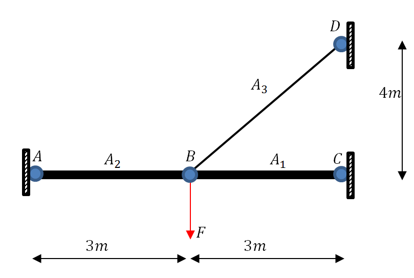
Most structural engineering problems in which the displacements and forces inside a structure are sought can be formulated using linear systems of equations. This is done by invoking certain assumptions that simplify the problem. However, when a structure undergoes large deformations, the problem has to be formulated using nonlinear systems of equations. The following is an example of a truss structure that aims at clarifying the difference.
Example
Two steel truss members with areas  and
and  are connected to a steel cable with an area
  as shown in the figure. All the connections are hinged connections allowing free relative rotations. Points
  ,
,  , and
, and  are fixed by means of hinges preventing displacements but allowing free rotations. Assuming that the horizontal displacement of point
  is
is  to the right and the vertical displacement of point is
  downwards. Assume that Young’s modulus
  ,
,  , and
, and  . The force in each member is equal to
  where
where  where
where  is the member number,
  is the undeformed length,
  is the deformed length,
  is the longitudinal stress,
  is the strain, and
  is Young’s modulus in member
  . Find the values of and at equilibrium using: 1) Linear analysis where the displacements are assumed to be small, and 2) Nonlinear analysis. Solve twice, once with
  , and another time with
  . Do the two solution strategies give the same answer?
Solution
The units adopted will be  for forces,
  for lengths, and
  for
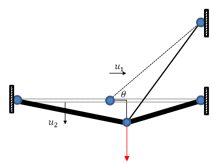
for  . The following is the displaced shape of the structure. The middle hinge move horizontally to the right a distance and vertically downards a distance . There are two unknowns in the problem and . These can be found using two equations of equilibrium at the middle hinge. The two equations are the sum of the vertical and horizontal forces, each equal to zero.
Linear Analysis
In linear analysis, the truss member length is assumed to only change due to displacements along its longitudinal axis. In other words, the forces in the truss member do not change if it simply rotates. In addition, the forces are assumed to be aligned with the original geometry of the structure before deformations. The strains in each member are given by:  ,
,  , and
, and  . Therefore, the forces in each member can be calculated as follows:
![\[ \begin{split} F_1&=E_1A_1\varepsilon_1=E\left(\frac{200}{1000000}\right)\frac{-u_1}{3}\\ F_2&=E_2A_2\varepsilon_2=E\left(\frac{200}{1000000}\right)\frac{u_1}{3}\\ F_3&=E_3A_3\varepsilon_3=E\left(\frac{50}{1000000}\right)\frac{u_2\sin{(\theta)}-u_1\cos{(\theta)}}{5} \end{split} \]](https://engcourses-uofa.ca/wp-content/ql-cache/quicklatex.com-fd39fcbc13056b5f73bdd6069e8a9d0d_l3.png "Rendered by QuickLaTeX.com")
where  ,
,  , and
, and  . Assuming small deformations, equilibrium at point can be analyzed using the following forces diagram:
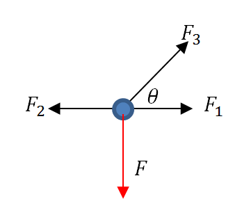
The first equation is the sum of horizontal forces equals to zero:
![\[ F_1+F_3\cos{(\theta)}-F_2=\frac{-81260000}{3}u_1+960000u_2=0 \]](https://engcourses-uofa.ca/wp-content/ql-cache/quicklatex.com-5a320c2e2515f31a9f2cfc39086e3845_l3.png "Rendered by QuickLaTeX.com")
The second equation is the sum of the vertical forces equal to zero:
![\[ F-F_3\sin{(\theta)}=F+960000u_1-1280000 u_2=0 \]](https://engcourses-uofa.ca/wp-content/ql-cache/quicklatex.com-c4eed18f5f9f9c152637314028281b53_l3.png "Rendered by QuickLaTeX.com")
These equations are linear and can be written in matrix form as follows:
![\[ \left(\begin{matrix} \frac{-81260000}{3} & 960000\\ 960000 & -1280000\end{matrix}\right)\left(\begin{array}{c} u_1\\u_2\end{array}\right)=\left(\begin{array}{c} 0\\-F\end{array}\right) \]](https://engcourses-uofa.ca/wp-content/ql-cache/quicklatex.com-eb8534d43fd151652eff3febefe60bd2_l3.png "Rendered by QuickLaTeX.com")
Setting yields a solution  and
and  , while setting
  yields
  and
and  . Notice that in a linear analysis, the displacements are directly proportional to the applied load, that is, the ratio between at
  and at is equal to
  . The same applies to .
The following is the Mathematica code to formulate and solve the above system of equations using the “Solve” function.
View Mathematica CodeClear[F, Ee];
Ee = 200 (10^9);
eps1 = -u1/3;
A1 = A2 = 200/1000000;
A3 = 50/1000000;
eps2 = u1/3;
Cth = 3/5;
Sth = 4/5;
eps3 = (-u1*Cth + u2*Sth)/5;
F1 = Ee*A1*eps1;
F2 = Ee*A2*eps2;
F3 = Ee*A3*eps3;
Eq1 = Expand[(F1 + F3*Cth - F2)]
Eq2 = Expand[F - F3*Sth]
sol1 = Solve[{Eq1 == 0.0, Eq2 == 0.0 /. F -> 10000}]
sol2 = Solve[{Eq1 == 0.0, Eq2 == 0.0 /. F -> 500000}]
import sympy as sp
sp.init_printing(use_latex=True)
u1, u2, F = sp.symbols('u1 u2 F')
Ee = 200*(10**9)
eps1 = -u1/3
A1 = A2 = 200/1000000
A3 = 50/1000000
eps2 = u1/3
Cth = 3/5
Sth = 4/5
eps3 = (-u1*Cth + u2*Sth)/5
F1 = Ee*A1*eps1
F2 = Ee*A2*eps2
F3 = Ee*A3*eps3
Eq1 = F1 + F3*Cth - F2
Eq2 = F - F3*Sth
display("Eq1: ",Eq1)
display("Eq2: ",Eq2)
# Using Sympy's built-in linear solve function
display("sol1: ",sp.linsolve((Eq1, Eq2.subs({'F':10000})),(u1, u2)))
display("sol2: ",sp.linsolve((Eq1, Eq2.subs({'F':500000})),(u1, u2)))
Nonlinear Analysis
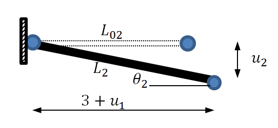
In a nonlinear analysis, the analysis takes into consideration the displaced position of the structure without any simplified assumptions. Looking at the first truss member, the displaced structure is shown in the following figure.
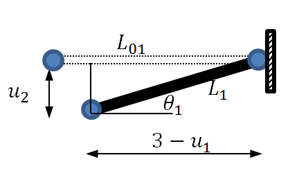
For this member, the original length  , the final length
  , the strain
  and the angle of inclination
  is such that
  and
and  .
.
For the second truss member, the displaced structure is shown in the following figure.
For this member, the original length  , the final length
  , the strain
  and the angle of inclination
  is such that
  and
and  .
.
For the third truss member, the displaced structure is shown in the following figure.
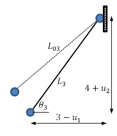
For this member, the original length  , the final length
  , the strain
  and the angle of inclination
  is such that
  and
and  .
.
Finally, the equations of equilibrium can be written taking into consideration the inclination of each member:
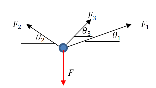
The first equation is the sum of horizontal forces equals to zero:
![\[ F_1\cos{(\theta_1)}+F_3\cos{(\theta_3)}-F_2\cos{(\theta_2)}=0 \]](https://engcourses-uofa.ca/wp-content/ql-cache/quicklatex.com-e8b9b4cca1f51f5df45bf744baff28d0_l3.png "Rendered by QuickLaTeX.com")
The second equation is the sum of the vertical forces equal to zero:
![\[ F-F_1\sin{(\theta_1)}-F_2\sin{(\theta_2)}-F_3\sin{(\theta_3)}=0 \]](https://engcourses-uofa.ca/wp-content/ql-cache/quicklatex.com-faba28b536a30b68b2037763ec643029_l3.png "Rendered by QuickLaTeX.com")
The following is a screenshot of the Mathematica output of the two equations:
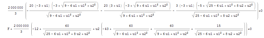
Setting yields a solution and , while setting yields  and
and  . For small deformations under small applied loads, the linear analysis and nonlinear analysis produce exactly the same results. In this situation, the rotations of the members are very small such that the original shape and the deformed shape can be assumed to be the same. However, under large loads, the linear analysis is no longer valid. The two solutions at are far from each other with the nonlinear analysis solution giving less displacement. In this particular situation, as the structure deforms, the nonlinear effects cause the structure to be more rigid and therefore exhibit less deformations. Cable structures with large loads and large deformations in the cables need to be analyzed using a nonlinear analysis rather than a linear analysis.
The following is the Mathematica code to formulate and solve the above nonlinear system of equations using the “FindRoot” function with an initial guess of  , and
, and  .
.
Ee = 200 (10^9);
A1 = A2 = 200/1000000;
A3 = 50/1000000;
L1 = Sqrt[(3 - u1)^2 + u2^2];
Sth1 = u2/L1;
Cth1 = (3 - u1)/L1;
L2 = Sqrt[(3 + u1)^2 + u2^2];
Sth2 = u2/L2;
Cth2 = (3 + u1)/L2;
L3 = Sqrt[(3 - u1)^2 + (4 + u2)^2];
Cth3 = (3 - u1)/L3;
Sth3 = (4 + u2)/L3;
eps1 = (L1 - 3)/3;
eps2 = (L2 - 3)/3;
eps3 = (L3 - 5)/5;
F1 = Ee*A1*eps1;
F2 = Ee*A2*eps2;
F3 = Ee*A3*eps3;
Eq1 = Simplify[F1*Cth1 - F2*Cth2 + F3*Cth3]
Eq2 = Simplify[F - F1*Sth1 - F2*Sth2 - F3*Sth3]

sol1 = FindRoot[{Eq1 == 0, Eq2 == 0 /. F -> 10000}, {{u1, 0}, {u2, 0}}]
sol2 = FindRoot[{Eq1 == 0, Eq2 == 0 /. F -> 500000}, {{u1, 0}, {u2, 0}}]
import sympy as sp
sp.init_printing(use_latex=True)
u1, u2, F = sp.symbols('u1 u2 F')
Ee = 200*(10**9)
A1 = A2 = 200/1000000
A3 = 50/1000000
L1 = sp.sqrt((3 - u1)**2 + u2**2)
Sth1 = u2/L1
Cth1 = (3 - u1)/L1
L2 = sp.sqrt((3 + u1)**2 + u2**2)
Sth2 = u2/L2
Cth2 = (3 + u1)/L2
L3 = sp.sqrt((3 - u1)**2 + (4 + u2)**2)
Cth3 = (3 - u1)/L3
Sth3 = (4 + u2)/L3
eps1 = (L1 - 3)/3
eps2 = (L2 - 3)/3
eps3 = (L3 - 5)/5
F1 = Ee*A1*eps1
F2 = Ee*A2*eps2
F3 = Ee*A3*eps3
Eq1 = F1*Cth1 - F2*Cth2 + F3*Cth3
Eq2 = F - F1*Sth1 - F2*Sth2 - F3*Sth3
display("Eq1: ",Eq1)
display("Eq2: ",Eq2)
# Using Sympy's built-in nonlinear solve function
display("sol1: ",sp.nsolve((Eq1, Eq2.subs({'F':10000})), (u1,u2), (0,0)))
display("sol2: ",sp.nsolve((Eq1, Eq2.subs({'F':500000})), (u1,u2), (0,0)))
At the end of linear analysis,
“the ratio between u1 at F=10,000 and u1 at F=500,000 is equal to 500,000/10,000.”
It should be
“the ratio between u1 at F=10,000 and u1 at F=500,000 is equal to 10,000/500,000.”
Corrected! Thank you!