Engineering at Alberta Courses » Quadratic Spline Interpolation

Piecewise Interpolation: Quadratic Spline Interpolation

Quadratic Spline Interpolation

For quadratic spline interpolation, we present two possible quadratic interpolation schemes.

Scheme 1:

In the first scheme, the intervals between the data points are used as intervals on which a quadratic function is defined. On the intermediate nodes, the slope of the parabola on the left is equated to the slope of the parabola on the right (Figure 3). Consider a set of $k$ data points $(x_1,y_1),(x_2,y_2),\cdots, (x_k,y_k)$ , with $k-1$ intervals. We seek to find a quadratic polynomial $s_i(x)=a_i+b_ix+c_ix^2$ on the $i^{th}$ interval $[x_i,x_{i+1}]$ . In total, there are $3(k-1)$ coefficients. On each interval, the two equations $s_i(x_i)=y_i$ and $s_i(x_{i+1})=y_{i+1}$ ensure that the spline passes through the data points which also ensure the continuity of the splines. These continuity equations will provide $2(k-1)$ equations. In addition, the connection of the quadratic polynomials at intermediate nodes will be assumed to be smooth, and so at every intermediate point the first derivative is assumed to be continuous, that is $s_i'(x_{i+1})=s_{i+1}'(x_{i+1})$ . These first-derivative continuity equations provide another $k-2$ equations. Finally, the second derivative at the starting point can be set to 0 to provide one additional condition so that the number of equations would be equal to $3(k-1)$ which is equal to the number of unknowns. The following are the resulting equations:

$\begin{split} a_1+b_1x_1+c_1x_1^2&=y_1\\ a_1+b_1x_2+c_1x_2^2&=y_2\\ a_2+b_2x_2+c_2x_2^2&=y_2\\ a_2+b_2x_3+c_2x_3^2&=y_3\\ \vdots&\\ a_{k-1}+b_{k-1}x_{k-1}+c_{k-1}x_{k-1}^2&=y_{k-1}\\ a_{k-1}+b_{k-1}x_k+c_{k-1}x_k^2&=y_k\\ b_1+2c_1x_2-b_2-2c_2x_2&=0\\ b_2+2c_2x_3-b_3-2c_3x_3&=0\\ \vdots&\\ b_{k-2}+2c_{k-2}x_{k-1}-b_{k-1}-2c_{k-1}x_{k-1}&=0\\ 2c_1&=0 \end{split}$

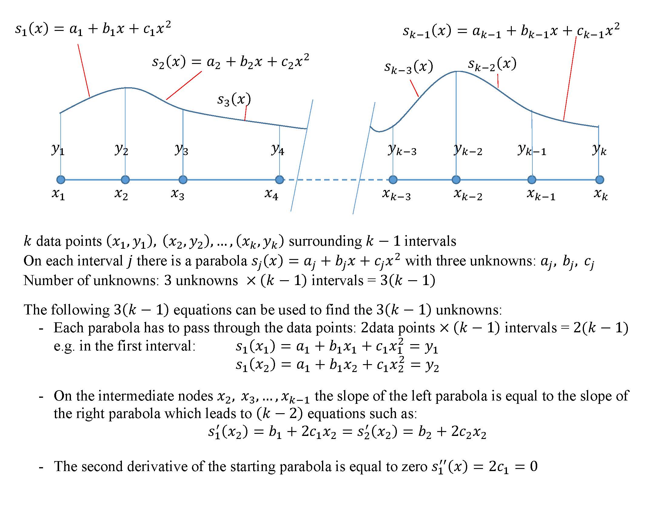
Figure 3. Scheme 1 of piecewise quadratic interpolation with continuity in the interpolating function and its first derivative

The following Mathematica code implements this procedure for a set of data (the procedure will only work if $x_1<x_2<\cdots<x_k$ ).

View Mathematica Code

Data = {{-1, 0.038}, {-0.8, 0.058}, {-0.60, 0.10}, {-0.4, 0.20}, {-0.2, 0.50}, {0, 1}, {0.2, 0.5}, {0.4, 0.2}, {0.6, 0.1}, {0.8, 0.058}, {1, 0.038}};
Spline2[Data_] := (k1 = Length[Data] - 1;
  y = Table[If[i <= 2 k1,If[EvenQ[i], Data[[i/2 + 1, 2]], Data[[(i + 1)/2, 2]]], 0], {i,1, 3 k1}];
  M = Table[0, {i, 1, 3 k1}, {j, 1, 3 k1}];
  For[i = 1, i <= k1, i = i + 1, 
   M[[2 i - 1, 3 (i - 1) + 1]] = M[[2 i, 3 (i - 1) + 1]] = 1; 
   M[[2 i - 1, 3 (i - 1) + 2]] = Data[[i, 1]]; 
   M[[2 i - 1, 3 (i - 1) + 1 + 2]] = Data[[i, 1]]^2; 
   M[[2 i, 3 (i - 1) + 1 + 1]] = Data[[i + 1, 1]]; 
   M[[2 i, 3 (i - 1) + 1 + 2]] = Data[[i + 1, 1]]^2];
  For[i = 1, i <= k1 - 1, i = i + 1, 
   M[[2 k1 + i, 3 (i - 1) + 1 + 1]] = 1; 
   M[[2 k1 + i, 3 (i - 1) + 1 + 4]] = -1; 
   M[[2 k1 + i, 3 (i - 1) + 1 + 2]] = 2 Data[[i + 1, 1]]; 
   M[[2 k1 + i, 3 (i - 1) + 1 + 5]] = -2 Data[[i + 1, 1]]];
  M[[3 k1, 3]] = 2;
  Coef = Inverse[M].y;
  pf = Table[{Coef[[3 (i - 1) + 1]] + Coef[[3 (i - 1) + 2]]*x + Coef[[3 (i - 1) + 3]]*x^2, Data[[i, 1]] <= x <= Data[[i + 1, 1]]}, {i, 1, k1}];
  Piecewise[pf])
y = Spline2[Data]
M // MatrixForm
yactual=1/(1+25x^2);
a = Plot[{y, yactual}, {x, -1, 1},Epilog -> {PointSize[Large], Point[Data]}, AxesLabel -> {"x", "y1"},ImageSize -> Medium, PlotRange -> All,PlotLegends -> {"y2", "yactual"}, PlotLabel ->"Quadratic spline"]

View Python Code

import numpy as np
import matplotlib.pyplot as plt

Data = [[-1, 0.038], [-0.8, 0.058], [-0.60, 0.10], [-0.4, 0.20], [-0.2, 0.50], [0, 1], [0.2, 0.5], [0.4, 0.2], [0.6, 0.1], [0.8, 0.058], [1, 0.038]]
def Spline2(x, Data):
  k1 = len(Data) - 1
  y = [(Data[i//2][1] if i%2==0 else Data[(i)//2][1]) if i <= 2*k1 else 0 for i in range(1, 3*k1 + 1)]
  M = np.zeros([3*k1, 3*k1])
  for i in range(k1):
    M[2*(i + 1) - 2][3*i] = M[2*(i + 1) - 1][3*i] = 1 
    M[2*(i + 1) - 2][3*i + 1] = Data[i][0] 
    M[2*(i + 1) - 2][3*i + 2] = Data[i][0]**2
    M[2*(i + 1) - 1][3*i + 1] = Data[i + 1][0] 
    M[2*(i + 1) - 1][3*i + 2] = Data[i + 1][0]**2
  for i in range(k1 - 1):
    M[2*k1 + i][3*i + 1] = 1
    M[2*k1 + i][3*i + 4] = -1 
    M[2*k1 + i][3*i + 2] = 2*Data[i + 1][0]
    M[2*k1 + i][3*i + 5] = -2*Data[i + 1][0]
  M[3*k1 - 1][2] = 2
  print("M Matrix\n", M)
  Coef = np.matmul(np.linalg.inv(M),y)
  display([['{:30}'.format(str(round(Coef[3*i],3)) + ' + ' + str(round(Coef[3*i + 1],3)) + 'x + ' + str(round(Coef[3*i + 2],3)) + 'x**2'),
            '{:15}'.format(str(round(Data[i][0],3))+' <=x<= '+str(round(Data[i + 1][0],3)))] for i in range(k1)])
  return np.piecewise(x, [(x >= Data[i][0])&(x <= Data[i + 1][0]) for i in range(k1)],
                         [lambda x, j=i: Coef[3*j] + Coef[3*j + 1]*x + Coef[3*j + 2]*x**2 for i in range(k1)])
x = np.arange(-1,1,0.01)
y = Spline2(x, Data)
yactual = 1/(1 + 25*x**2)
plt.plot(x,yactual, label="yactual")
plt.plot(x, y, label="y2")
plt.scatter([point[0] for point in Data],[point[1] for point in Data], c='k')
plt.title("Quadratic spline")
plt.xlabel("x"); plt.ylabel("y2")
plt.legend(); plt.grid(); plt.show()

The following MATLAB code applies scheme 1 to data extracted from the Runge function:

MATLAB files: File 1 (ex8_3.m)File 2 (spline2a.m)

Example

Use scheme 1 of quadratic interpolation to find the interpolating function given the following 4 data points (-1, 0.038) (-0.8, 0.058), (-0.60, 0.10), (-0.4, 0.20)

Solution

The four data points ( $k=4$ ) with three intervals ( $k-1=3$ ), therefore, there are $3(k-1)=9$ unknowns. The following are the nine equations according to scheme 1 to be solved to find the unknowns:

$\begin{split} a_1+b_1(-1)+c_1(-1)^2&=0.038\\ a_1+b_1(-0.8)+c_1(-0.8)^2&=0.058\\ a_2+b_2(-0.8)+c_2(-0.8)^2&=0.058\\ a_2+b_2(-0.6)+c_2(-0.6)^2&=0.10\\ a_3+b_3(-0.6)+c_3(-0.6)^2&=0.10\\ a_3+b_3(-0.4)+c_3(-0.4)^2&=0.20\\ b_1+2c_1(-0.8)-b_2-2c_2(-0.8)&=0\\ b_2+2c_2(-0.6)-b_3-2c_3(-0.6)&=0\\ 2c_1&=0 \end{split}$

Solving the above equations produces the following interpolation function:

$y=\begin{cases}s_1(x)=0.138+0.1x,&-1\leq x<-0.8\\ s_2(x)=0.49+0.98x+0.55x^2, &-0.8 \leq x<-0.6\\ s_3(x)=0.616 + 1.4 x + 0.9 x^2, & -0.6 \leq x \leq -0.4 \end{cases}$

Figure 4 shows the resulting interpolation function along with the four data points. The Mathematica code is provided below the figure.

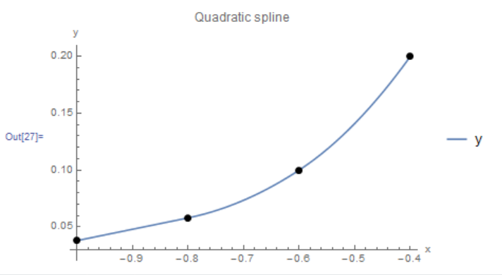
Figure 4. Scheme 1 quadratic interpolation applied to four data points

View Mathematica Code

Data = {{-1, 0.038}, {-0.8, 0.058}, {-0.60, 0.10}, {-0.4, 0.20}};
Spline2[Data_] := (k1 = Length[Data] - 1;
  y = Table[
    If[i <= 2 k1, 
     If[EvenQ[i], Data[[i/2 + 1, 2]], Data[[(i + 1)/2, 2]]], 0], {i, 
     1, 3 k1}];
  M = Table[0, {i, 1, 3 k1}, {j, 1, 3 k1}];
  For[i = 1, i <= k1, i = i + 1, 
   M[[2 i - 1, 3 (i - 1) + 1]] = M[[2 i, 3 (i - 1) + 1]] = 1;
   M[[2 i - 1, 3 (i - 1) + 2]] = Data[[i, 1]];
   M[[2 i - 1, 3 (i - 1) + 1 + 2]] = Data[[i, 1]]^2;
   M[[2 i, 3 (i - 1) + 1 + 1]] = Data[[i + 1, 1]];
   M[[2 i, 3 (i - 1) + 1 + 2]] = Data[[i + 1, 1]]^2];
  For[i = 1, i <= k1 - 1, i = i + 1, 
   M[[2 k1 + i, 3 (i - 1) + 1 + 1]] = 1;
   M[[2 k1 + i, 3 (i - 1) + 1 + 4]] = -1;
   M[[2 k1 + i, 3 (i - 1) + 1 + 2]] = 2 Data[[i + 1, 1]];
   M[[2 k1 + i, 3 (i - 1) + 1 + 5]] = -2 Data[[i + 1, 1]]];
  M[[3 k1, 3]] = 2;
  Coef = Inverse[M].y;
  pf = Table[{Coef[[3 (i - 1) + 1]] + Coef[[3 (i - 1) + 2]]*x + Coef[[3 (i - 1) + 3]]*x^2, Data[[i, 1]] <= x <= Data[[i + 1, 1]]}, {i, 1, k1}];
  Piecewise[pf])
y = Spline2[Data]
M // MatrixForm
a = Plot[{y}, {x, -1, -0.4}, Epilog -> {PointSize[Large], Point[Data]}, AxesLabel -> {"x", "y2"},ImageSize -> Medium, PlotRange -> All, PlotLegends -> {"y2"}, PlotLabel -> "Quadratic spline"]

View Python Code

import numpy as np
import matplotlib.pyplot as plt

Data = [[-1, 0.038], [-0.8, 0.058], [-0.60, 0.10], [-0.4, 0.20]]
def Spline2(x, Data):
  k1 = len(Data) - 1
  y = [(Data[i//2][1] if i%2==0 else Data[(i)//2][1]) if i <= 2*k1 else 0 for i in range(1, 3*k1 + 1)]
  M = np.zeros([3*k1, 3*k1])
  for i in range(k1):
    M[2*(i + 1) - 2][3*i] = M[2*(i + 1) - 1][3*i] = 1 
    M[2*(i + 1) - 2][3*i + 1] = Data[i][0] 
    M[2*(i + 1) - 2][3*i + 2] = Data[i][0]**2
    M[2*(i + 1) - 1][3*i + 1] = Data[i + 1][0] 
    M[2*(i + 1) - 1][3*i + 2] = Data[i + 1][0]**2
  for i in range(k1 - 1):
    M[2*k1 + i][3*i + 1] = 1
    M[2*k1 + i][3*i + 4] = -1 
    M[2*k1 + i][3*i + 2] = 2*Data[i + 1][0]
    M[2*k1 + i][3*i + 5] = -2*Data[i + 1][0]
  M[3*k1 - 1][2] = 2
  print("M Matrix\n", M)
  Coef = np.matmul(np.linalg.inv(M),y)
  display([['{:30}'.format(str(round(Coef[3*i],3)) + ' + ' + str(round(Coef[3*i + 1],3)) + 'x + ' + str(round(Coef[3*i + 2],3)) + 'x**2'),
            '{:15}'.format(str(round(Data[i][0],3))+' <=x<= '+str(round(Data[i + 1][0],3)))] for i in range(k1)])
  return np.piecewise(x, [(x >= Data[i][0])&(x <= Data[i + 1][0]) for i in range(k1)],
                         [lambda x, j=i: Coef[3*j] + Coef[3*j + 1]*x + Coef[3*j + 2]*x**2 for i in range(k1)])
x = np.arange(-1,-0.4,0.01)
y = Spline2(x, Data)
plt.plot(x, y, label="y2")
plt.scatter([point[0] for point in Data],[point[1] for point in Data], c='k')
plt.title("Quadratic spline")
plt.xlabel("x"); plt.ylabel("y2")
plt.legend(); plt.grid(); plt.show()

The following MATLAB code applies scheme 1 to the data from this example:

MATLAB files:File 1 (ex8_2.m)File 2 (spline2b.m)

Disadvantages

In certain cases, such as fluctuating data, this scheme might lead to some oscillations within the intervals between the data points. As an example, when this scheme is used to fit through the 11 data points of the Runge function given in the previous section, a nice smooth interpolating function is produced for the first few intervals (Figure 5). The condition of having zero second derivative $s_1''(x_1)=0$ on the initial interval causes the interpolating in the first interval to follow the line connecting the first two data points. However, in the last five intervals, the interpolating function oscillates and deviates away from the expected behaviour.

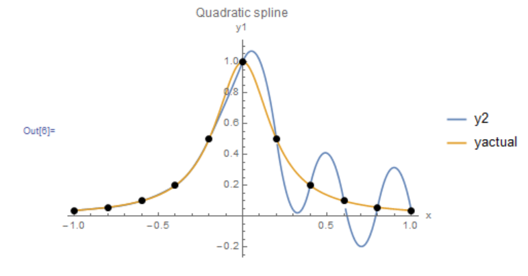
Figure 5. Behaviour of scheme 1 for quadratic interpolation of the Runge function data points.

Scheme 2

For the second scheme, the intervals where the quadratic interpolation functions are defined, are chosen different from the intervals between the data points in a manner to ensure symmetry of the quadratic interpolation. The new intervals where the piecewise quadratic functions are defined are bounded by the points $x_1<\frac{x_2+x_3}{2}<\frac{x_3+x_4}{2}<\cdots<\frac{x_{k-2}+x_{k-1}}{2}<x_k$ (Figure 6). Consider a set of $k$ data points $(x_1,y_1),(x_2,y_2),\cdots, (x_k,y_k)$ , with $k-1$ intervals. On each of the $k-2$ intervals bounded by $x_1<\frac{x_2+x_3}{2}<\frac{x_3+x_4}{2}<\cdots<\frac{x_{k-2}+x_{k-1}}{2}<x_k$ a quadratic polynomial $s_i(x)=a_i+b_ix+c_ix^2$ is defined. In total, there are $3(k-2)$ coefficients. First,the quadratic polynomials have to pass through the $k$ data poitns resulting in $k$ equations. These quadratic polynomials have to be continuous and differentiable at the $k-3$ intermediate points that are the bounds of the intervals resulting in $2(k-3)$ equations. Therefore, in total, there are $3(k-2)$ equations which is equal to the number of unknowns. The following are the resulting equations:

$\begin{split} a_1+b_1x_1+c_1x_1^2&=y_1\\ a_1+b_1x_2+c_1x_2^2&=y_2\\ a_2+b_2x_3+c_2x_3^2&=y_3\\a_3+b_3x_4+c_3x_4^2&=y_4\\ \vdots&\\ a_{k-2}+b_{k-2}x_{k-1}+c_{k-2}x_{k-1}^2&=y_{k-1}\\ a_{k-2}+b_{k-2}x_k+c_{k-2}x_k^2&=y_k\\ \vdots&\\ a_1+b_1\left(\frac{x_2+x_3}{2}\right)+c_1\left(\frac{x_2+x_3}{2}\right)^2&=a_2+b_2\left(\frac{x_2+x_3}{2}\right)+c_2\left(\frac{x_2+x_3}{2}\right)^2\\ a_2+b_2\left(\frac{x_3+x_4}{2}\right)+c_2\left(\frac{x_3+x_4}{2}\right)^2&=a_3+b_3\left(\frac{x_3+x_4}{2}\right)+c_3\left(\frac{x_3+x_4}{2}\right)^2\\ a_{k-3}+b_{k-3}\left(\frac{x_{k-2}+x_{k-1}}{2}\right)+c_{k-3}\left(\frac{x_{k-2}+x_{k-1}}{2}\right)^2&=\\ a_{k-2}+b_{k-2}\left(\frac{x_{k-2}+x_{k-1}}{2}\right)&+c_{k-2}\left(\frac{x_{k-2}+x_{k-1}}{2}\right)^2\\ b_1+2c_1\left(\frac{x_2+x_3}{2}\right)-b_2-2c_2\left(\frac{x_2+x_3}{2}\right)&=0\\ b_2+2c_2\left(\frac{x_3+x_4}{2}\right)-b_3-2c_3\left(\frac{x_3+x_4}{2}\right)&=0\\ \vdots&\\ b_{k-3}+2c_{k-3}\left(\frac{x_{k-2}+x_{k-1}}{2}\right)-b_{k-2}-2c_{k-2}&\left(\frac{x_{k-2}+x_{k-1}}{2}\right)=0 \end{split}$

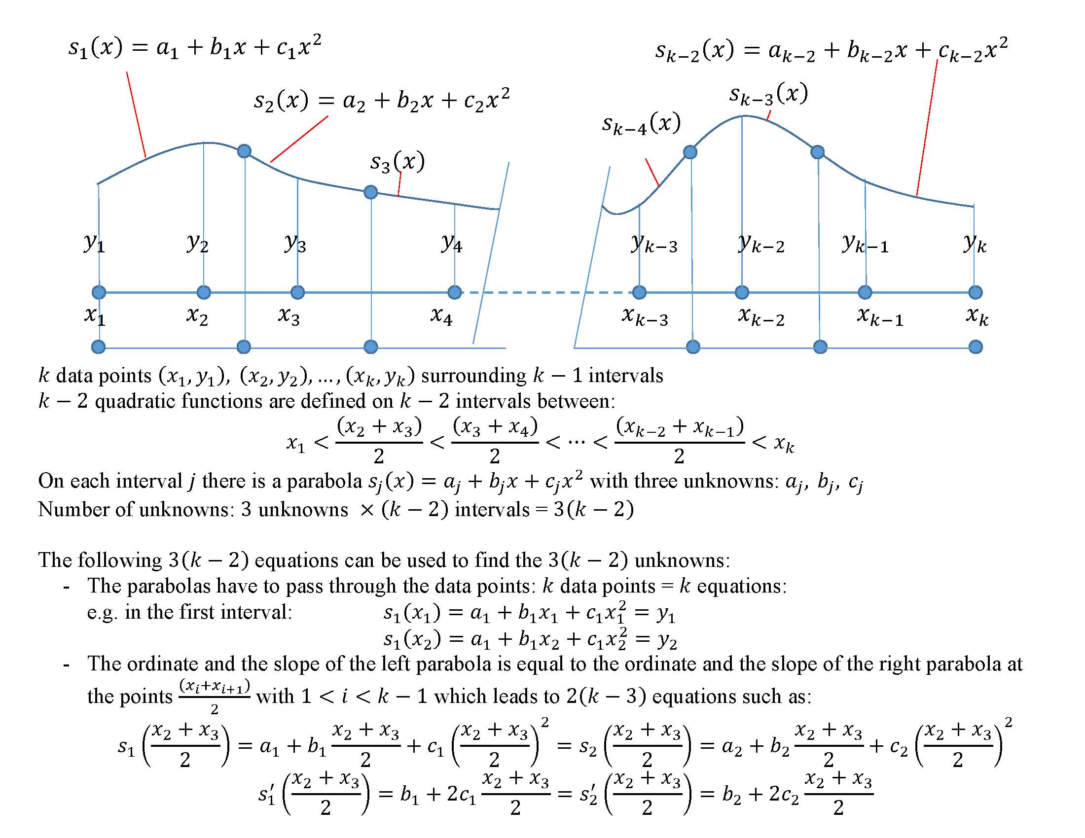
Figure 6. Scheme 2 of piecewise quadratic interpolation with continuity in the interpolating function and its first derivative

The following Mathematica code implements this procedure for a set of data (the procedure will only work if $x_1<x_2<\cdots<x_k$ ). As shown in Figure 7, the oscillations produced by scheme 1 disappear if this scheme is used for interpolating the data points of the Runge function given in the previous section.

View Mathematica Code

Data = {{-1, 0.038}, {-0.8, 0.058}, {-0.60, 0.10}, {-0.4,0.20}, {-0.2, 0.50}, {0, 1}, {0.2, 0.5}, {0.4, 0.2}, {0.6,0.1}, {0.8, 0.058}, {1, 0.038}};
Spline2[Data_] := (k = Length[Data];
  NewData = Table[0, {i, 1, k - 3}];
  Do[NewData[[i]] = (Data[[i + 1]] + Data[[i + 2]])/2, {i, 1, k - 3}];
  NNewData = Prepend[Append[NewData, Data[[k]]], Data[[1]]];
  y = Table[If[i <= k - 1 + 1, Data[[i, 2]], 0], {i, 1, 3 k - 6}];
  M = Table[0, {i, 1, 3 k - 6}, {j, 1, 3 k - 6}];
  M[[1, 1]] = M[[2, 1]] = 1;
  M[[1, 2]] = Data[[1, 1]];
  M[[1, 3]] = Data[[1, 1]]^2;
  M[[2, 2]] = Data[[2, 1]];
  M[[2, 3]] = Data[[2, 1]]^2;
  M[[k - 1, 3 k - 8]] = M[[k, 3 k - 8]] = 1;
  M[[k - 1, 3 k - 7]] = Data[[k - 1, 1]];
  M[[k - 1, 3 k - 6]] = Data[[k - 1, 1]]^2;
  M[[k, 3 k - 7]] = Data[[k, 1]];
  M[[k, 3 k - 6]] = Data[[k, 1]]^2;
  For[i = 3, i <= k - 2, i = i + 1, M[[i, 3 (i - 2) + 1]] = 1; 
   M[[i, 3 (i - 2) + 2]] = Data[[i, 1]]; 
   M[[i, 3 (i - 2) + 3]] = Data[[i, 1]]^2];
  For[i = 1, i <= k - 3, i = i + 1,
   M[[k + i, 3 (i - 1) + 1]] = 1; M[[k + i, 3 (i - 1) + 4]] = -1; 
   M[[k + i, 3 (i - 1) + 2]] = NewData[[i, 1]]; 
   M[[k + i, 3 (i - 1) + 5]] = -NewData[[i, 1]]; 
   M[[k + i, 3 (i - 1) + 3]] = NewData[[i, 1]]^2; 
   M[[k + i, 3 (i - 1) + 6]] = -1*NewData[[i, 1]]^2;
   M[[k + i + k - 3, 3 (i - 1) + 2]] = 1; 
   M[[k + i + k - 3, 3 (i - 1) + 5]] = -1; 
   M[[k + i + k - 3, 3 (i - 1) + 3]] = 2*NewData[[i, 1]]; 
   M[[k + i + k - 3, 3 (i - 1) + 6]] = -2*NewData[[i, 1]]];
  Coef = Inverse[M].y;
  pf = Table[{Coef[[3 (i - 1) + 1]] + Coef[[3 (i - 1) + 2]]*x + Coef[[3 (i - 1) + 3]]*x^2,NNewData[[i, 1]] <= x <= NNewData[[i + 1, 1]]}, {i, 1, k - 2}];
  Piecewise[pf])
y = Spline2[Data]
yactual = 1/(1 + 25 x^2);
M//MatrixForm
a = Plot[{y, yactual}, {x, -1, 1}, Epilog -> {PointSize[Large], Point[Data]}, AxesLabel -> {"x", "y2"},ImageSize -> Medium, PlotRange -> All, PlotLegends -> {"y2", "yactual"}, PlotLabel -> "Quadratic spline"]

View Python Code

import numpy as np
import matplotlib.pyplot as plt

Data = [[-1, 0.038], [-0.8, 0.058], [-0.60, 0.10], [-0.4, 0.20], [-0.2, 0.50], [0, 1], [0.2, 0.5], [0.4, 0.2], [0.6,0.1], [0.8, 0.058], [1, 0.038]]
def Spline2(x, Data):
  k = len(Data)
  Data = np.array(Data)
  NewData = np.array([(Data[i + 1] + Data[i + 2])/2 for i in range(k-3)])
  NNewData = np.vstack([Data[0], NewData, Data[k-1]])
  y = [Data[i][1] if i < k else 0 for i in range(3*k - 6)]
  M = np.zeros([3*k - 6, 3*k - 6])
  M[0][0] = M[1][0] = 1
  M[0][1] = Data[0][0]
  M[0][2] = Data[0][0]**2
  M[1][1] = Data[1][0]
  M[1][2] = Data[1][0]**2
  M[k - 2][3*k - 9] = M[k - 1][3*k - 9] = 1
  M[k - 2][3*k - 8] = Data[k - 2][0]
  M[k - 2][3*k - 7] = Data[k - 2][0]**2
  M[k - 1][3*k - 8] = Data[k - 1][0]
  M[k - 1][3*k - 7] = Data[k - 1][0]**2
  for i in range(2, k-2):
    M[i][3*(i - 1)] = 1
    M[i][3*(i - 1) + 1] = Data[i][0] 
    M[i][3*(i - 1) + 2] = Data[i][0]**2
  for i in range(k - 3):
    M[k + i][3*i] = 1
    M[k + i][3*i + 3] = -1
    M[k + i][3*i + 1] = NewData[i][0]
    M[k + i][3*i + 4] = -NewData[i][0] 
    M[k + i][3*i + 2] = NewData[i][0]**2 
    M[k + i][3*i + 5] = -1*NewData[i][0]**2
    M[k + i + k - 3][3*i + 1] = 1
    M[k + i + k - 3][3*i + 4] = -1 
    M[k + i + k - 3][3*i + 2] = 2*NewData[i][0] 
    M[k + i + k - 3][3*i + 5] = -2*NewData[i][0]
  print("M Matrix\n", M)
  Coef = np.matmul(np.linalg.inv(M),y)
  display([['{:30}'.format(str(round(Coef[3*i],3)) + ' + ' + str(round(Coef[3*i + 1],3)) + 'x + ' + str(round(Coef[3*i + 2],3)) + 'x**2'),
            '{:15}'.format(str(round(NNewData[i][0],3))+' <=x<= '+str(round(NNewData[i + 1][0],3)))] for i in range(k - 2)])
  return np.piecewise(x, [(x >= NNewData[i][0])&(x <= NNewData[i + 1][0]) for i in range(k - 2)],
                         [lambda x, j=i: Coef[3*j] + Coef[3*j + 1]*x + Coef[3*j + 2]*x**2 for i in range(k - 2)])
x = np.arange(-1,1,0.01)
yactual = 1/(1 + 25*x**2)
y = Spline2(x, Data)
plt.plot(x, yactual, label="yactual")
plt.plot(x, y, label="y2")
plt.scatter([point[0] for point in Data],[point[1] for point in Data], c='k')
plt.title("Quadratic spline")
plt.xlabel("x"); plt.ylabel("y2")
plt.legend(); plt.grid(); plt.show()

The following MATLAB code applies scheme 2 to data extracted from the Runge function:

MATLAB fileDownload

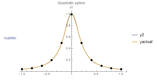
Figure 7. Behaviour of scheme 2 of quadratic interpolation when applied to the Runge function data points

Example

Use scheme 2 of quadratic interpolation to find the interpolating function given the following 5 data points (-1, 0.038) (-0.8, 0.058), (-0.60, 0.10), (-0.4, 0.20), (-0.2, 0.5)

Solution

The five data points ( $k=5$ ) with four intervals ( $k-1=4$ ). $k-2=3$ intervals for the quadratic interpolation functions are defined between the points $-1<-0.7<-0.5<-0.2$ . Therefore, there are $3(k-2)=9$ unknowns. The following are the nine equations according to scheme 2 to be solved to find the unknowns:

$\begin{split} a_1+b_1(-1)+c_1(-1)^2&=0.038\\ a_1+b_1(-0.8)+c_1(-0.8)^2&=0.058\\ a_2+b_2(-0.6)+c_2(-0.6)^2&=0.10\\ a_3+b_3(-0.4)+c_3(-0.4)^2&=0.20\\ a_3+b_3(-0.2)+c_3(-0.2)^2&=0.5\\ a_1+b_1(-0.7)+c_1(-0.7)^2&=a_2+b_2(-0.7)+c_2(-0.7)^2\\ a_2+b_2(-0.5)+c_2(-0.5)^2&=a_3+b_3(-0.5)+c_3(-0.5)^2\\ b_1+2c_1(-0.7)-b_2-2c_2(-0.7)&=0\\ b_2+2c_2(-0.5)-b_3-2c_3(-0.5)&=0\\ \end{split}$

Solving the above equations produces the following interpolation function:

$y=\begin{cases}s_1(x)=0.336857 + 0.547429 x + 0.248571 x^2,&-1\leq x<-0.7\\ s_2(x)=0.440457 + 0.843429 x + 0.46 x^2, &-0.7 \leq x<-0.5\\ s_3(x)=1.02331 + 3.17486 x + 2.79143 x^2, & -0.5\leq x\leq -0.2 \end{cases}$

Figure 8 shows the resulting interpolation function along with the five data points. The Mathematica code is provided below the figure.

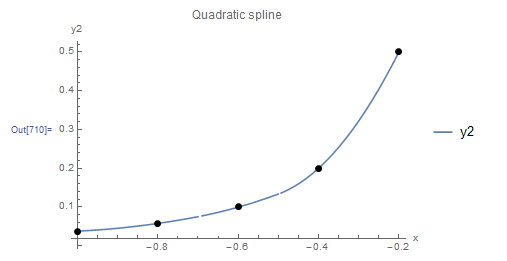
Figure 8. Scheme 1 quadratic interpolation applied to five data points

Figure 8. Scheme 2 quadratic interpolation applied to five data points

View Mathematica Code

Data = {{-1, 0.038}, {-0.8, 0.058}, {-0.60, 0.10}, {-0.4,0.20}, {-0.2, 0.50}};
Spline2[Data_] := (k = Length[Data];
  NewData = Table[0, {i, 1, k - 3}];
  Do[NewData[[i]] = (Data[[i + 1]] + Data[[i + 2]])/2, {i, 1, k - 3}];
  NNewData = Prepend[Append[NewData, Data[[k]]], Data[[1]]];
  y = Table[If[i <= k - 1 + 1, Data[[i, 2]], 0], {i, 1, 3 k - 6}];
  M = Table[0, {i, 1, 3 k - 6}, {j, 1, 3 k - 6}];
  M[[1, 1]] = M[[2, 1]] = 1;
  M[[1, 2]] = Data[[1, 1]];
  M[[1, 3]] = Data[[1, 1]]^2;
  M[[2, 2]] = Data[[2, 1]];
  M[[2, 3]] = Data[[2, 1]]^2;
  M[[k - 1, 3 k - 8]] = M[[k, 3 k - 8]] = 1;
  M[[k - 1, 3 k - 7]] = Data[[k - 1, 1]];
  M[[k - 1, 3 k - 6]] = Data[[k - 1, 1]]^2;
  M[[k, 3 k - 7]] = Data[[k, 1]];
  M[[k, 3 k - 6]] = Data[[k, 1]]^2;
  For[i = 3, i <= k - 2, i = i + 1, M[[i, 3 (i - 2) + 1]] = 1;
   M[[i, 3 (i - 2) + 2]] = Data[[i, 1]];
   M[[i, 3 (i - 2) + 3]] = Data[[i, 1]]^2];
  For[i = 1, i <= k - 3, i = i + 1, M[[k + i, 3 (i - 1) + 1]] = 1; 
   M[[k + i, 3 (i - 1) + 4]] = -1;
   M[[k + i, 3 (i - 1) + 2]] = NewData[[i, 1]];
   M[[k + i, 3 (i - 1) + 5]] = -NewData[[i, 1]];
   M[[k + i, 3 (i - 1) + 3]] = NewData[[i, 1]]^2;
   M[[k + i, 3 (i - 1) + 6]] = -1*NewData[[i, 1]]^2;
   M[[k + i + k - 3, 3 (i - 1) + 2]] = 1;
   M[[k + i + k - 3, 3 (i - 1) + 5]] = -1;
   M[[k + i + k - 3, 3 (i - 1) + 3]] = 2*NewData[[i, 1]];
   M[[k + i + k - 3, 3 (i - 1) + 6]] = -2*NewData[[i, 1]]];
  Coef = Inverse[M].y;
  pf = Table[{Coef[[3 (i - 1) + 1]] + Coef[[3 (i - 1) + 2]]*x + Coef[[3 (i - 1) + 3]]*x^2, NNewData[[i, 1]] <= x <= NNewData[[i + 1, 1]]}, {i, 1, k - 2}];
  Piecewise[pf])
y = Spline2[Data]
M // MatrixForm
a = Plot[{y}, {x, -1, -0.2}, Epilog -> {PointSize[Large], Point[Data]}, AxesLabel -> {"x", "y2"}, ImageSize -> Medium, PlotRange -> All, PlotLegends -> {"y2"},  PlotLabel -> "Quadratic spline"]

View Python Code

import numpy as np
import matplotlib.pyplot as plt

Data = [[-1, 0.038], [-0.8, 0.058], [-0.60, 0.10], [-0.4,0.20], [-0.2, 0.50]]
def Spline2(x, Data):
  k = len(Data)
  Data = np.array(Data)
  NewData = np.array([(Data[i + 1] + Data[i + 2])/2 for i in range(k-3)])
  NNewData = np.vstack([Data[0], NewData, Data[k-1]])
  y = [Data[i][1] if i < k else 0 for i in range(3*k - 6)]
  M = np.zeros([3*k - 6, 3*k - 6])
  M[0][0] = M[1][0] = 1
  M[0][1] = Data[0][0]
  M[0][2] = Data[0][0]**2
  M[1][1] = Data[1][0]
  M[1][2] = Data[1][0]**2
  M[k - 2][3*k - 9] = M[k - 1][3*k - 9] = 1
  M[k - 2][3*k - 8] = Data[k - 2][0]
  M[k - 2][3*k - 7] = Data[k - 2][0]**2
  M[k - 1][3*k - 8] = Data[k - 1][0]
  M[k - 1][3*k - 7] = Data[k - 1][0]**2
  for i in range(2, k-2):
    M[i][3*(i - 1)] = 1
    M[i][3*(i - 1) + 1] = Data[i][0] 
    M[i][3*(i - 1) + 2] = Data[i][0]**2
  for i in range(k - 3):
    M[k + i][3*i] = 1
    M[k + i][3*i + 3] = -1
    M[k + i][3*i + 1] = NewData[i][0]
    M[k + i][3*i + 4] = -NewData[i][0] 
    M[k + i][3*i + 2] = NewData[i][0]**2 
    M[k + i][3*i + 5] = -1*NewData[i][0]**2
    M[k + i + k - 3][3*i + 1] = 1
    M[k + i + k - 3][3*i + 4] = -1 
    M[k + i + k - 3][3*i + 2] = 2*NewData[i][0] 
    M[k + i + k - 3][3*i + 5] = -2*NewData[i][0]
  print("M Matrix\n", M)
  Coef = np.matmul(np.linalg.inv(M),y)
  display([['{:30}'.format(str(round(Coef[3*i],3)) + ' + ' + str(round(Coef[3*i + 1],3)) + 'x + ' + str(round(Coef[3*i + 2],3)) + 'x**2'),
            '{:15}'.format(str(round(NNewData[i][0],3))+' <=x<= '+str(round(NNewData[i + 1][0],3)))] for i in range(k - 2)])
  return np.piecewise(x, [(x >= NNewData[i][0])&(x <= NNewData[i + 1][0]) for i in range(k - 2)],
                         [lambda x, j=i: Coef[3*j] + Coef[3*j + 1]*x + Coef[3*j + 2]*x**2 for i in range(k - 2)])
x = np.arange(-1,-0.2,0.01)
y = Spline2(x, Data)
plt.plot(x, y, label="y2")
plt.scatter([point[0] for point in Data],[point[1] for point in Data], c='k')
plt.title("Quadratic spline")
plt.xlabel("x"); plt.ylabel("y2")
plt.legend(); plt.grid(); plt.show()

The following MATLAB code applies scheme 2 to the data from this example:

MATLAB fileDownload

Open Educational Resources

Piecewise Interpolation: Quadratic Spline Interpolation

Quadratic Spline Interpolation

Scheme 1:

Example

Solution

Disadvantages

Scheme 2

Example

Solution

Lecture Video

Leave a Reply Cancel reply