Engineering at Alberta Courses » Cubic Spline Interpolation

Piecewise Interpolation: Cubic Spline Interpolation

Cubic Spline Interpolation

There are different schemes of piecewise cubic spline interpolation functions which vary according to the end conditions. The scheme presented here is sometimes referred to as “Not-a-knot” end condition in which the first cubic spline is defined over the interval $x\in [x_1,x_3)$ and the last cubic spline is defined on the interval $x\in[x_{k-2},x_k]$ (Figure 9). Given $k$ data points with $k-1$ intervals, $k-3$ cubic polynomials are defined on the intervals: $x_1<x_3<x_4<\cdots<x_{k-3}<x_{k-2}<x_k$ . $\forall i \leq k-3$ each cubic polynomial is defined as: $s_i(x)=a_i+b_ix+c_ix^2+d_ix^3$ . The $4(k-3)$ unknowns can be obtained using the following conditions(Figure 9):

Each polynomial has to pass through the data points which are the bounds of the interval, therefore this results in $2(k-3)$ equations. In addition the first polynomial and the last ( $k-3$ ) polynomial have to pass through the second and next-to-last data points respectively. In total, this produces $2(k-3)+2$ equations.
On the $k-4$ intermediate nodes between the polynomials, the first and second derivatives are equal to each other. This results in $2(k-4)$ equations

The above system of equations is guaranteed a unique solution as long as the data points are ordered: $x_1<x_2<\cdots<x_k$ .

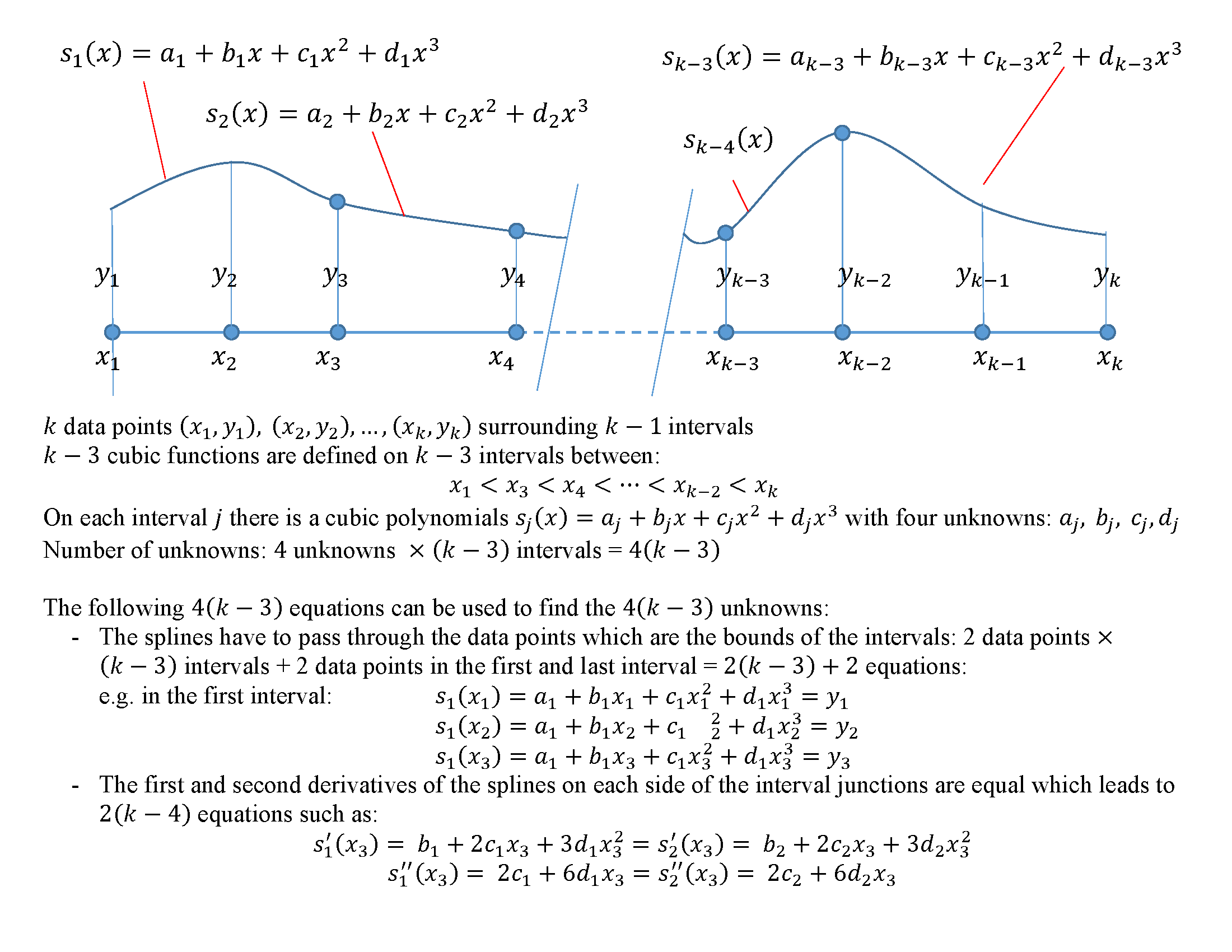
Figure 9. Scheme of piecewise cubic interpolation with continuity in the first and second derivatives.

The following Mathematica code implements this procedure for a set of data (the procedure will only work if $x_1<x_2<\cdots<x_k$ ).

As shown in Figure 10, this cubic interpolation scheme produces a very smooth interpolating function for the data points of the Runge function given in the previous section.

View Mathematica Code

Data = {{-1, 0.038}, {-0.8, 0.058}, {-0.60, 0.10}, {-0.4,0.20}, {-0.2, 0.50}, {0, 1}, {0.2, 0.5}, {0.4, 0.2}, {0.6, 0.1}, {0.8, 0.058}, {1, 0.038}};
Clear[x, a, b, c, d]
Spline3[Data_] := (k = Length[Data];
  atable = Table[Subscript[a, i], {i, 1, k - 3}];
  btable = Table[Subscript[b, i], {i, 1, k - 3}];
  ctable = Table[Subscript[c, i], {i, 1, k - 3}];
  dtable = Table[Subscript[d, i], {i, 1, k - 3}];
  Poly = Table[atable[[i]] + btable[[i]]*x + ctable[[i]]*x^2 + dtable[[i]]*x^3, {i, 1, k - 3}];
  intermediate = Table[Data[[i + 2]], {i, 1, k - 4}];
  Equations = Table[0, {i, 1, 4 (k - 3)}];
  Do[Equations[[i]] = (Poly[[i]] /. x -> Data[[i + 2, 1]]) == Data[[i + 2, 2]], {i, 1, k - 4}];
  Do[Equations[[i + k - 4]] = (Poly[[i + 1]] /. x -> Data[[i + 2, 1]]) == Data[[i + 2, 2]], {i, 1, k - 4}];
  Equations[[2 (k - 4) + 1]] = (Poly[[1]] /. x -> Data[[1, 1]]) == Data[[1, 2]];
  Equations[[2 (k - 4) + 2]] = (Poly[[1]] /. x -> Data[[2, 1]]) == Data[[2, 2]];
  Equations[[2 (k - 4) + 3]] = (Poly[[k - 3]] /. x -> Data[[k - 1, 1]]) == Data[[k - 1, 2]];
  Equations[[2 (k - 4) + 4]] = (Poly[[k - 3]] /. x -> Data[[k, 1]]) == Data[[k, 2]];
  Do[Equations[[2 (k - 3) + 2 + i]] = (D[Poly[[i]], x] /.  x -> intermediate[[i, 1]]) == (D[Poly[[i + 1]], x] /.  x -> intermediate[[i, 1]]), {i, 1, k - 4}];
  Do[Equations[[2 (k - 3) + 2 + k - 4 + i]] = (D[Poly[[i]], {x, 2}] /. x -> intermediate[[i, 1]]) == (D[Poly[[i + 1]], {x, 2}] /.x -> intermediate[[i, 1]]), {i, 1, k - 4}];
  un = Flatten[{atable, btable, ctable, dtable}];
  f = Solve[Equations];
  Poly = Poly /. f[[1]];
  xs = intermediate;
  xs = Prepend[Append[xs, Data[[k]]], Data[[1]]];
  pf = Table[{Poly[[i]], xs[[i, 1]] <= x <= xs[[i + 1, 1]]}, {i, 1, k - 3}];
  Piecewise[pf])
y = Spline3[Data]
yactual = 1/(1 + 25 x^2);
a = Plot[y, {x, -1, 1}, Epilog -> {PointSize[Large], Point[Data]}, AxesLabel -> {"x", "y3"}, ImageSize -> Medium, PlotRange -> All,  PlotLegends -> {"y3"}, PlotLabel -> "cubic spline"]
a = Plot[{y, yactual}, {x, -1, 1},  Epilog -> {PointSize[Large], Point[Data]}, AxesLabel -> {"x", "y3"}, ImageSize -> Medium, PlotRange -> All,  PlotLegends -> {"y3", "yactual"}, PlotLabel -> "cubic spline"]

View Python Code

import numpy as np
import sympy as sp
import matplotlib.pyplot as plt

Data = [[-1, 0.038], [-0.8, 0.058], [-0.60, 0.10], [-0.4,0.20], [-0.2, 0.50], [0, 1], [0.2, 0.5], [0.4, 0.2], [0.6, 0.1], [0.8, 0.058], [1, 0.038]]
def Spline3(x_val, Data):
  k = len(Data)
  a,b,c,d = sp.symbols('a:d', cls=sp.Function)
  x = sp.symbols('x')
  atable = [a(i) for i in range(k - 3)]
  btable = [b(i) for i in range(k - 3)]
  ctable = [c(i) for i in range(k - 3)]
  dtable = [d(i) for i in range(k - 3)]
  Poly = [atable[i] + btable[i]*x + ctable[i]*x**2 + dtable[i]*x**3 for i in range(k - 3)]
  intermediate = [Data[i + 2] for i in range(k - 4)]
  Equations = [0 for i in range(4*(k - 3))]
  for i in range(k - 4):
    Equations[i] = (Poly[i].subs(x, Data[i + 2][0])) - Data[i + 2][1]
  for i in range(k - 4):
    Equations[i + k - 4] = (Poly[i + 1].subs(x, Data[i + 2][0])) - Data[i + 2][1]
  Equations[2*(k - 4)] = (Poly[0].subs(x, Data[0][0])) - Data[0][1]
  Equations[2*(k - 4) + 1] = (Poly[0].subs(x, Data[1][0])) - Data[1][1]
  Equations[2*(k - 4) + 2] = (Poly[k - 4].subs(x, Data[k - 2][0])) - Data[k - 2][1]
  Equations[2*(k - 4) + 3] = (Poly[k - 4].subs(x, Data[k - 1][0])) - Data[k - 1][1]
  for i in range(k - 4):
    Equations[2*(k - 3) + i + 2] = (Poly[i].diff(x).subs(x, intermediate[i][0])) - (Poly[i + 1].diff(x).subs(x, intermediate[i][0]))
  for i in range(k - 4):
    Equations[2*(k - 2) + k + i - 4] = (Poly[i].diff(x, 2).subs(x, intermediate[i][0])) - (Poly[i + 1].diff(x, 2).subs(x, intermediate[i][0]))
  un = atable + btable + ctable + dtable
  f = list(sp.linsolve(Equations, un))
  vars = {}
  for i in range(len(un)):
    vars[un[i]] = f[0][i];
  Poly = [Poly[i].subs(vars) for i in range(len(Poly))]
  xs = np.vstack([Data[0], intermediate, Data[k - 1]])
  display([['{:45}'.format(str(sp.N(Poly[i],4))),
            '{:15}'.format(str(round(xs[i][0],3))+' <=x<= '+str(round(xs[i + 1][0],3)))] for i in range(k - 3)])
  return np.piecewise(x_val, [(x_val >= xs[i][0])&(x_val <= xs[i + 1][0]) for i in range(len(Poly))],
                             [sp.lambdify(x, Poly[i]) for i in range(len(Poly))])
  
x = np.arange(-1, 1, 0.01)
y = Spline3(x, Data)
yactual = 1/(1 + 25*x**2)
plt.plot(x, yactual, label="yactual")
plt.plot(x, y, label="y3")
plt.scatter([point[0] for point in Data],[point[1] for point in Data], c='k')
plt.title("Cubic spline")
plt.xlabel("x"); plt.ylabel("y3")
plt.legend(); plt.grid(); plt.show()

The following MATLAB code fits a cubic spline interpolation function to data extracted using the Runge function:

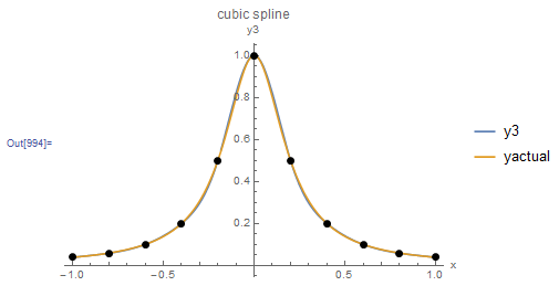
MATLAB files: File 1 (ex8_4b.m)File 2 (spline3.m)

Figure 10. Behaviour of the cubic spline interpolation scheme when applied to the Runge function data points

Example

Use the cubic spline interpolation scheme presented above to find the interpolating function given the following 5 data points (-1, 0.038) (-0.8, 0.058), (-0.60, 0.10), (-0.4, 0.20), (-0.2, 0.5)

Solution

There are $k=5$ data points, therefore, there are $k-3=5-3=2$ cubic polynomials required for interpolation. These are:

$y=\begin{cases}a_1+b_1x+c_1x^2+d_1x^3,&-1\leq x < -0.6\\ a_2+b_2x+c_2x^2+d_2x^3,&-0.6\leq x \leq -0.2 \end{cases}$

To find the associated $4(2)=8$ unknown coefficients, the following system of 8 linear equations is solved:

$\begin{split} a_1-0.6b_1+0.36c_1-0.216d_1&=0.1\\ a_2-0.6b_2+0.36c_2-0.216d_2&=0.1\\ a_1-b_1+c_1-d_1&=0.038\\ a_1-0.8b_1+0.64c_1-0.512d_1&=0.058\\ a_2-0.4b_2+0.16c_2-0.064d_2&=0.2\\ a_2-0.2b_2+0.04c_2-0.008d_2&=0.5\\ b_1-1.2c_1+1.08d_1&=b_2-1.2c_2+1.08d_2\\ 2c_1-3.6d_1&=2c_2-3.6d_2 \end{split}$

Solving the above system, yields the following interpolation function:

$y=\begin{cases}0.453+0.967083x+0.75x^2+0.197917x^3,&-1\leq x < -0.6\\ 1.1685+4.54458x+6.7125x^2+3.51042x^3,&-0.6\leq x \leq -0.2 \end{cases}$

Figure 11 shows the resulting interpolation function along with the five data points. The Mathematica code is provided below the figure.

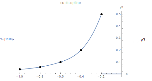
Figure 11. Cubic spline interpolation applied to five data points.

View Mathematica Code

Data = {{-1, 0.038}, {-0.8, 0.058}, {-0.60, 0.10}, {-0.4,  0.20}, {-0.2, 0.50}};
Clear[x, a, b, c, d]
Spline3[Data_] := (k = Length[Data];
  atable = Table[Subscript[a, i], {i, 1, k - 3}];
  btable = Table[Subscript[b, i], {i, 1, k - 3}];
  ctable = Table[Subscript[c, i], {i, 1, k - 3}];
  dtable = Table[Subscript[d, i], {i, 1, k - 3}];
  Poly = Table[atable[[i]] + btable[[i]]*x + ctable[[i]]*x^2 + dtable[[i]]*x^3, {i, 1, k - 3}];
  intermediate = Table[Data[[i + 2]], {i, 1, k - 4}];
  Equations = Table[0, {i, 1, 4 (k - 3)}];
  Do[Equations[[i]] = (Poly[[i]] /. x -> Data[[i + 2, 1]]) ==      Data[[i + 2, 2]], {i, 1, k - 4}];
  Do[Equations[[i + k - 4]] = (Poly[[i + 1]] /. x -> Data[[i + 2, 1]]) == Data[[i + 2, 2]], {i, 1, k - 4}];
  Equations[[2 (k - 4) + 1]] = (Poly[[1]] /. x -> Data[[1, 1]]) ==  Data[[1, 2]];
  Equations[[2 (k - 4) + 2]] = (Poly[[1]] /. x -> Data[[2, 1]]) ==  Data[[2, 2]];
  Equations[[2 (k - 4) + 3]] = (Poly[[k - 3]] /.  x -> Data[[k - 1, 1]]) == Data[[k - 1, 2]];
  Equations[[2 (k - 4) + 4]] = (Poly[[k - 3]] /. x -> Data[[k, 1]]) == Data[[k, 2]];
  Do[Equations[[2 (k - 3) + 2 + i]] = (D[Poly[[i]], x] /. x -> intermediate[[i, 1]]) == (D[Poly[[i + 1]], x] /. x -> intermediate[[i, 1]]), {i, 1, k - 4}];
  Do[Equations[[2 (k - 3) + 2 + k - 4 + i]] = (D[Poly[[i]], {x, 2}] /. x -> intermediate[[i, 1]]) == (D[Poly[[i + 1]], {x, 2}] /.  x -> intermediate[[i, 1]]), {i, 1, k - 4}];
  f = Solve[Equations];
  Poly = Poly /. f[[1]];
  xs = intermediate;
  xs = Prepend[Append[xs, Data[[k]]], Data[[1]]];
  pf = Table[{Poly[[i]], xs[[i, 1]] <= x <= xs[[i + 1, 1]]}, {i, 1, k - 3}];
  Piecewise[pf])
Equations // MatrixForm
y = Spline3[Data]
a = Plot[y, {x, -1, 0}, Epilog -> {PointSize[Large], Point[Data]}, AxesLabel -> {"x", "y3"}, ImageSize -> Medium, PlotRange -> All,  PlotLegends -> {"y3"}, PlotLabel -> "cubic spline"]

View Python Code

import numpy as np
import sympy as sp
import matplotlib.pyplot as plt

Data = [[-1, 0.038], [-0.8, 0.058], [-0.60, 0.10], [-0.4,  0.20], [-0.2, 0.50]]
def Spline3(x_val, Data):
  k = len(Data)
  a,b,c,d = sp.symbols('a:d', cls=sp.Function)
  x = sp.symbols('x')
  atable = [a(i) for i in range(k - 3)]
  btable = [b(i) for i in range(k - 3)]
  ctable = [c(i) for i in range(k - 3)]
  dtable = [d(i) for i in range(k - 3)]
  Poly = [atable[i] + btable[i]*x + ctable[i]*x**2 + dtable[i]*x**3 for i in range(k - 3)]
  intermediate = [Data[i + 2] for i in range(k - 4)]
  Equations = [0 for i in range(4*(k - 3))]
  for i in range(k - 4):
    Equations[i] = (Poly[i].subs(x, Data[i + 2][0])) - Data[i + 2][1]
  for i in range(k - 4):
    Equations[i + k - 4] = (Poly[i + 1].subs(x, Data[i + 2][0])) - Data[i + 2][1]
  Equations[2*(k - 4)] = (Poly[0].subs(x, Data[0][0])) - Data[0][1]
  Equations[2*(k - 4) + 1] = (Poly[0].subs(x, Data[1][0])) - Data[1][1]
  Equations[2*(k - 4) + 2] = (Poly[k - 4].subs(x, Data[k - 2][0])) - Data[k - 2][1]
  Equations[2*(k - 4) + 3] = (Poly[k - 4].subs(x, Data[k - 1][0])) - Data[k - 1][1]
  for i in range(k - 4):
    Equations[2*(k - 3) + i + 2] = (Poly[i].diff(x).subs(x, intermediate[i][0])) - (Poly[i + 1].diff(x).subs(x, intermediate[i][0]))
  for i in range(k - 4):
    Equations[2*(k - 2) + k + i - 4] = (Poly[i].diff(x, 2).subs(x, intermediate[i][0])) - (Poly[i + 1].diff(x, 2).subs(x, intermediate[i][0]))
  un = atable + btable + ctable + dtable
  f = list(sp.linsolve(Equations, un))
  vars = {}
  for i in range(len(un)):
    vars[un[i]] = f[0][i];
  Poly = [Poly[i].subs(vars) for i in range(len(Poly))]
  xs = np.vstack([Data[0], intermediate, Data[k - 1]])
  display([['{:45}'.format(str(sp.N(Poly[i],4))),
            '{:15}'.format(str(round(xs[i][0],3))+' <=x<= '+str(round(xs[i + 1][0],3)))] for i in range(k - 3)])
  return np.piecewise(x_val, [(x_val >= xs[i][0])&(x_val <= xs[i + 1][0]) for i in range(len(Poly))],
                             [sp.lambdify(x, Poly[i]) for i in range(len(Poly))])
  
x = np.arange(-1, -0.2, 0.001)
y = Spline3(x, Data)
yactual = 1/(1 + 25*x**2)
plt.plot(x, yactual, label="yactual")
plt.plot(x, y, label="y3")
plt.scatter([point[0] for point in Data],[point[1] for point in Data], c='k')
plt.title("Cubic spline")
plt.xlabel("x"); plt.ylabel("y3")
plt.legend(); plt.grid(); plt.show()

The following MATLAB code fits a cubic spline interpolation function to the data from this example:

MATLAB fileDownload

Open Educational Resources

Piecewise Interpolation: Cubic Spline Interpolation

Cubic Spline Interpolation

Example

Solution

Lecture Video

Leave a Reply Cancel reply