Engineering at Alberta Courses » Romberg’s Method

Numerical Integration: Romberg’s Method

Romberg’s Method

Richardson Extrapolation

Romberg’s method applied a technique called the Richardson extrapolation to the trapezoidal integration rule (and can be applied to any of the rules above). The general Richardson extrapolation technique is a powerful method that combines two or more less accurate solutions to obtain a highly accurate one. The essential ingredient of the method is the knowledge of the order of the truncation error. Assuming a numerical technique approximates the value of $A$ by choosing the value of $h_1$ , and calculating an estimate $A^*(h_1)$ according to the equation:

$A=A^*(h_1)+C(h_1^{k_1})+\mathcal{O}(h_1^{k_2})$

Where $C$ is a constant whose value does not need to be known and $k_2\geq k_1+1$ . If a smaller $h_2 < h_1$ is chosen with $t=\frac{h_1}{h_2}$ , then the new estimate for $A$ is $A^*(h_2)$ and the equation becomes:

$A=A^*(h_2)+C(h_2^{k_1})+\mathcal{O}(h_2^{k_2})$

Multiplying the second equation by $t^{k_1}$ and subtracting the first equation yields:

$(t^{k_1}-1)A=t^{k_1}A^*(h_2)-A^*(h_1)+\mathcal{O}(h_1^{k_2})$

Therefore:

$A=\frac{(t^{k_1}A^*(h_2)-A^*(h_1))}{(t^{k_1}-1)}+\mathcal{O}(h_1^{k_2})$

In other words, if the first error term in a method is directly proportional to $h^{k_1}$ , then, by combining two values of $h$ , we can get an estimate whose error term is directly proportional to $h^{k_2}$ . The above equation can also be written as:

$A=\frac{(t^{k_1}A^*\left(\frac{h_1}{t}\right)-A^*(h_1))}{(t^{k_1}-1)}+\mathcal{O}(h_1^{k_2})$

Romberg’s Method Using the Trapezoidal Rule

As shown above the truncation error in the trapezoidal rule is $\mathcal{O}(h^{2})$ . If the trapezoidal numerical integration scheme is applied for a particular value of $h_1$ and then applied again for half that value (i.e., $t=\frac{h_1}{h_2}=2$ ), then, substituting in the equation above yields:

$I=\frac{\left(2^{2}I_T\left(\frac{h_1}{2}\right)-I_T(h_1)\right)}{(2^{2}-1)}+\mathcal{O}(h_1^{k_2})=\frac{4I_T\left(\frac{h_1}{2}\right)-I_T(h_1)}{3}+\mathcal{O}(h_1^{k_2})$

It should be noted that for the trapezoidal rule, $k_2$ is equal to 4, i.e., the error term using this method is $\mathcal{O}(h_1^4)$ . To explicitly observe this, consider the error analysis for the trapezoidal rule. As proved in the section of Trapezoidal Rule, the error analysis led to the following expression,

$\begin{split} \int_a^b f(x)\mathrm dx &=\frac{h}{2}\Big ( f(a) + f(b) +2\sum_{j=1}^{n-1} f(x_j)\Big )\\ & - (b-a)\frac{h^2}{12}f''(\xi)- (b-a)\frac{h^4}{480}f^{(4)}(\eta) + \cdots \end{split}$

Letting $A=I:=\int_a^b f(x)\mathrm dx$ , $A^*(h)=I_T(h):=\frac{h}{2}\left ( f(a) + f(b) +2\sum_{j=1}^{n-1} f(x_j)\right )$ , $k_1=2$ and $k_2=4$ , we can write:

$I=\frac{(t^{k_1}I^*\left(\frac{h_1}{t}\right)-I^*(h_1))}{(t^{k_1}-1)}+\mathcal{O}(h_1^{k_2})=\frac{(t^{2}I^*\left(\frac{h_1}{2}\right)-I^*(h_1))}{(t^{2}-1)}+\mathcal{O}(h_1^{k_4})$

showing that the error term is $\mathcal{O}(h_1^{k_4})$ .

This method can be applied successively by halving the value of $h$ to obtain an error estimate that is $\mathcal{O}(h_1^6)$ . Assuming that the trapezoidal integration is available for $h_1$ , $\frac{h_1}{2}$ , $\frac{h_1}{4}$ , and $\frac{h_1}{8}$ , then the first two can be used to find an estimate $I_{T1}$ that is $\mathcal{O}(h_1^{4})$ , and the last two can be used to find an estimate $I_{T2}$ that is $\mathcal{O}\left(\left(\frac{h_1}{4}\right)^{4}\right)$ . Applying the Richardson extrapolation equation to $I_{T1}$ and $I_{T2}$ and noticing that $t=4$ in this case produce the following estimate for $I$ :

$I=\frac{\left(4^{2}I_{T2}-I_{T1}\right)}{(4^{2}-1)}+\mathcal{O}(h_1^{6})=\frac{16I_{T2}-I_{T1}}{15}+\mathcal{O}(h_1^{6})$

The process can be extended even further to find an estimate that is $\mathcal{O}(h_1^{8})$ . In general, the process can be written as follows:

$I_{j,k}=\frac{\left(2^{2(k-1)}I_{j+1,k-1}-I_{j,k-1}\right)}{(2^{2(k-1)}-1)}+\mathcal{O}(h_1^{2k})$

where $j+1$ indicates the more accurate integral, while $j$ indicates the less accurate integral, $k=1,2,3,\cdots$ correspond to the calculations with error terms that correspond to $h^2, h^4, h^6,\cdots$ , respectively. The above equation is applied for $k\geq 2$ . For example, setting $k=2$ and $j=1$ yields:

$I_{1,2}=\frac{4I_{2,1}-I_{1,1}}{3}+\mathcal{O}(h_1^{4})$

Similarly, setting $k=3$ and $j=1$ yields:

$I_{1,3}=\frac{\left(16I_{2,2}-I_{1,2}\right)}{15}+\mathcal{(O)}(h_1^{6})$

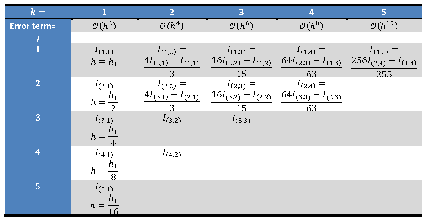
The following table sketches how the process is applied to obtain an estimate that is $\mathcal{O}(h^{10})$ using this algorithm. The first column corresponds to evaluating the integral for the values of $h$ , $\frac{h}{2}$ , $\frac{h}{4}$ , $\frac{h}{8}$ , and $\frac{h}{16}$ . These correspond to $n$ , $2n$ , $4n$ , $8n$ , and $16n$ trapezoids, respectively. The equation above is then used to fill the remaining values in the table.

A stopping criterion for this algorithm can be set as:

$\varepsilon_r=\left|\frac{I_{1,k}-I_{1,k-1}}{I_{1,k}}\right|\leq \varepsilon_s$

The following Mathematica code provides a procedural implementation of the Romberg’s method using the trapezoidal rule. The first procedure “IT[f,a,b,n]” provides the numerical estimate for the integral of $f$ from $a$ to $b$ with $n$ being the number of trapezoids. The “RI[f,a,b,k,n1]” procedure builds the Romberg’s method table shown above up to $k$ columns. $n_1$ provides the number of subdivisions (number of trapezoids) in the first entry in the table $I_{1,1}$ .

View Mathematica Code

IT[f_, a_, b_, n_] := (h = (b - a)/n; Sum[(f[a + (i - 1)*h] + f[a + i*h])*h/2, {i, 1, n}])
RI[f_, a_, b_, k_,n1_] := (RItable = Table["N/A", {i, 1, k}, {j, 1, k}];
Do[RItable[[i, 1]] = IT[f, a, b, 2^(i - 1)*n1], {i, 1, k}];
  Do[RItable[[j, ik]] = (2^(2 (ik - 1)) RItable[[j + 1, ik - 1]] - RItable[[j, ik - 1]])/(2^(2 (ik - 1)) - 1), {ik, 2, k}, {j, 1,k - ik + 1}];
  ERtable =  Table[(RItable[[1, i + 1]] - RItable[[1, i]])/RItable[[1, i + 1]], {i, 1, k - 1}];
  {RItable, ERtable})
a = 0.0;
b = 2;
k=3;
n1=1;
f[x_] := E^x
Integrate[f[x], {x, a, b}]
s = RI[f, a, b, k,n1];
s[[1]] // MatrixForm
s[[2]] // MatrixForm

View Python Code

import numpy as np
from scipy import integrate

def IT(f, a, b, n):
  h = (b - a)/n
  return sum([(f(a + i*h) + f(a + (i + 1)*h))*h/2 for i in range(n)])
def RI(f, a, b, k, n1):
  RItable = [[None for i in range(k)] for j in range(k)]
  for i in range(k):
    RItable[i][0] = IT(f, a, b, 2**i*n1)
  for ik in range(1, k):
    for j in range(k - ik):
      RItable[j][ik] = (2**(2*ik)*RItable[j + 1][ik - 1] - RItable[j][ik - 1])/(2**(2*ik) - 1)
  ERtable =  [(RItable[0][i + 1] - RItable[0][i])/RItable[0][i + 1] for i in range(k - 1)]
  return [RItable, ERtable]
a = 0.0
b = 2
k = 3
n1 = 1
def f(x): return np.exp(x)
y, error = integrate.quad(f, a, b)
print("Integrate: ",y)
s = RI(f, a, b, k,n1)
display("RItable:",s[0])
display("ERtable:",s[1])

Example 1

As shown in the example above in the trapezoidal rule, when 71 trapezoids were used, the estimate for the integral of $e^x$ from $a=0$ to $b=2$ was $I_T=6.38948$ with an absolute error of $|E|=0.00042$ . Using the Romberg’s method, find the depth $k$ starting with $h_1=b-a=2$ so that the estimate for the same integral has the same or less absolute error $|E|\leq 0.00042$ . Compare the number of computations required by the Romberg’s method to that required by the traditional trapezoidal rule to obtain an estimate with the same absolute error.

Solution

First, we will start with $k=2$ . For that, we will need to compute the integral numerically using the trapezoidal rule for a chosen $h_1$ and then for $\frac{h_1}{2}$ to fill in the entries $I_{1,1}$ and $I_{2,1}$ in the Romberg’s method table.

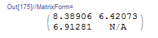
Assuming $h_1=b-a=2$ , i.e., 1 trapezoid, the value of $I_{1,1}=8.38906$ . Assuming a trapezoid width of $\frac{h_1}{2}=1$ , i.e., two trapezoids on the interval, the value of $I_{2,1}=6.91281$ . Using the Romberg table, the value of $I_{1,2}$ can be computed as:

$I_{1,2}=\frac{4I_{2,1}-I_{1,1}}{3}=6.42073$

with a corresponding absolute error of $|E|=|6.42073-6.38906|=0.0317>0.00042$ .
The output Romberg table with depth $k=2$ has the following form:
RT1

Next, to fill in the table up to depth $k=3$ , the value of $I_{3,1}$ in the table needs to be calculated. This value corresponds to the calculation of the trapezoidal rule with a trapezoid width of $\frac{h_1}{2^{k-1}}=\frac{h_1}{4}$ , i.e., 4 trapezoids on the whole interval. Using the trapezoidal rule, we get $I_{3,1}=6.52161$ . The remaining values in the Romberg table can be calculated as follows:

$\begin{split} I_{2,2}&=\frac{4I_{3,1}-I_{2,1}}{3}=\frac{4\times 6.52161-6.91281}{3}=6.39121\\ I_{1,3}&=\frac{16I_{2,2}-I_{1,2}}{15}=\frac{16\times 6.39121-6.42073}{15}=6.38924\\ \end{split}$

with the absolute error in $I_{1,3}$ that is less than the specified error: $|E|=|6.38924-6.38906|=0.000186<0.00042$ . The output Romberg table with depth $k=3$ has the following form: RT2

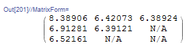
Number of Computations

For the same error, the traditional trapezoidal rule would have required 71 trapezoids. If we assume each trapezoid is one computation, the Romberg’s method requires computations of 1 trapezoid in $I_{1,1}$ , two trapezoids in $I_{2,1}$ , and 4 trapezoids in $I_{3,1}$ with a total of 7 corresponding computations. I.e., almost one tenth of the computational resources is required by the Romberg’s method in this example to produce the same level of accuracy!

The following Mathematica code was used to produce the above calculations.

View Mathematica Code

IT[f_, a_, b_, n_] := (h = (b - a)/n;  Sum[(f[a + (i - 1)*h] + f[a + i*h])*h/2, {i, 1, n}])
RI[f_, a_, b_, k_, n1_] := (RItable = Table["N/A", {i, 1, k}, {j, 1, k}];
  Do[RItable[[i, 1]] = IT[f, a, b, 2^(i - 1)*n1], {i, 1, k}];
  Do[RItable[[j,ik]] = (2^(2 (ik - 1)) RItable[[j + 1, ik - 1]] - RItable[[j, ik - 1]])/(2^(2 (ik - 1)) - 1), {ik, 2, k}, {j, 1, k - ik + 1}];
  ERtable = Table[(RItable[[1, i + 1]] - RItable[[1, i]])/RItable[[1, i + 1]], {i, 1, k - 1}];
  {RItable, ERtable})
a = 0.0;
b = 2;
(*Depth of Romberg Table*)
k = 3;
n1 = 1;
f[x_] := E^x
Itrue = Integrate[f[x], {x, a, b}]
s = RI[f, a, b, k, n1];
s[[1]] // MatrixForm
s[[2]] // MatrixForm
ErrorTable = Table[If[RItable[[i, j]] == "N/A", "N/A", Abs[Itrue - RItable[[i, j]]]], {i, 1, Length[RItable]}, {j, 1, Length[RItable]}];
ErrorTable // MatrixForm

View Python Code

import numpy as np
from scipy import integrate

def IT(f, a, b, n):
  h = (b - a)/n
  return sum([(f(a + i*h) + f(a + (i + 1)*h))*h/2 for i in range(int(n))])
def RI(f, a, b, k, n1):
  RItable = [[None for i in range(k)] for j in range(k)]
  for i in range(k):
    RItable[i][0] = IT(f, a, b, 2**i*n1)
  for ik in range(1, k):
    for j in range(k - ik):
      RItable[j][ik] = (2**(2*ik)*RItable[j + 1][ik - 1] - RItable[j][ik - 1])/(2**(2*ik) - 1)
  ERtable =  [(RItable[0][i + 1] - RItable[0][i])/RItable[0][i + 1] for i in range(k - 1)]
  return [RItable, ERtable]
a = 0.0
b = 2
# Depth of Romberg Table
k = 3
n1 = 1
def f(x): return np.exp(x)
Itrue, error = integrate.quad(f, a, b)
print("Itrue: ",Itrue)
s = RI(f, a, b, k, n1)
RItable = s[0]
display("RItable:",s[0])
display("ERtable:",s[1])
ErrorTable = [[None if RItable[i][j] == None else abs(Itrue - RItable[i][j]) for j in range(len(RItable))] for i in range(len(RItable))]
display("ErrorTable",ErrorTable)

MATLAB files: File 1 (ex11_6.m) File 2 (trap_func.m)

Example 2

Consider the integral:

$I=\int_{0}^{1.5}\! 2 + 2 x + x^2 + \sin{(2 \pi x)} + \cos{(2 \pi \frac{x}{0.5})}\,\mathrm{d}x$

Using the trapezoidal rule, draw a table with the following columns: $n$ , $h$ , $I_T$ , $I_{true}$ , and $|E|$ , where $n$ is the number of trapezoids, $h$ is the width of each trapezoid, $I_T$ is the estimate using the trapezoidal rule, $I_{true}$ is the true value of the integral, and $|E|$ is the absolute value of the error. Use $n=1, 2, 4, 8, 16,\cdots,128$ . Similarly, provide the Romberg table with depth $k=5$ . Compare the number of computations in each and the level of accuracy.

Solution

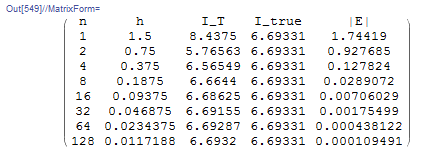
The true value of the integral can be computed using Mathematica as $I_{\mbox{true}}=6.69331$ . For the trapezoidal rule, the following Mathematica code is used to produce the required table for the specified values of $n$ :

View Mathematica Code

IT[f_, a_, b_, n_] := (h = (b - a)/n;   Sum[(f[a + (i - 1)*h] + f[a + i*h])*h/2, {i, 1, n}])
a = 0.0;
b = 1.5;
f[x_] := 2 + 2 x + x^2 + Sin[2 Pi*x] + Cos[2 Pi*x/0.5]
Title = {"n", "h", "I_T", "I_true", "|E|"};
Ii = Table[{2^(i - 1), (b - a)/2^(i - 1), ss = IT[f, a, b, 2^(i - 1)], Itrue, Abs[Itrue - ss]}, {i, 1, 8}];
Ii = Prepend[Ii, Title];
Ii // MatrixForm

View Python Code

import numpy as np
import pandas as pd
from scipy import integrate

def IT(f, a, b, n):
  h = (b - a)/n
  return sum([(f(a + i*h) + f(a + (i + 1)*h))*h/2 for i in range(int(n))])
a = 0.0
b = 1.5
def f(x): return 2 + 2*x + x**2 + np.sin(2*np.pi*x) + np.cos(2*np.pi*x/0.5)
Itrue, error = integrate.quad(f, a, b)
Ii = []
for i in range(8):
  ss = IT(f, a, b, 2**i)
  Ii.append([2**i, (b - a)/2**i, ss, Itrue, abs(Itrue - ss)])
Ii = pd.DataFrame(Ii, columns=["n", "h", "I_T", "I_true", "|E|"])
display(Ii)

The table shows that with 128 subdivisions, the value of the absolute error is 0.00011.
RT3

For the Romberg table, the code developed above is used to produce the following table:

View Mathematica Code

IT[f_, a_, b_, n_] := (h = (b - a)/n; Sum[(f[a + (i - 1)*h] + f[a + i*h])*h/2, {i, 1, n}])
RI[f_, a_, b_, k_, n1_] := (RItable = Table["N/A", {i, 1, k}, {j, 1, k}];
  Do[RItable[[i, 1]] = IT[f, a, b, 2^(i - 1)*n1], {i, 1, k}];
  Do[RItable[[j, ik]] = (2^(2 (ik - 1)) RItable[[j + 1, ik - 1]] - RItable[[j, ik - 1]])/(2^(2 (ik - 1)) - 1), {ik, 2, k}, {j, 1,  k - ik + 1}];
  ERtable =  Table[(RItable[[1, i + 1]] - RItable[[1, i]])/ RItable[[1, i + 1]], {i, 1, k - 1}];
  {RItable, ERtable})
a = 0.0;
b = 1.5;
k = 5;
n1 = 1;
f[x_] := 2 + 2 x + x^2 + Sin[2 Pi*x] + Cos[2 Pi*x/0.5]
Itrue = Integrate[f[x], {x, a, b}]
s = RI[f, a, b, k, n1];
s[[1]] // MatrixForm
s[[2]] // MatrixForm
ErrorTable = Table[If[RItable[[i, j]] == "N/A", "N/A", Abs[Itrue - RItable[[i, j]]]], {i, 1, Length[RItable]}, {j, 1,  Length[RItable]}];
ErrorTable // MatrixForm

View Python Code

import numpy as np
from scipy import integrate

def IT(f, a, b, n):
  h = (b - a)/n
  return sum([(f(a + i*h) + f(a + (i + 1)*h))*h/2 for i in range(int(n))])
def RI(f, a, b, k, n1):
  RItable = [[None for i in range(k)] for j in range(k)]
  for i in range(k):
    RItable[i][0] = IT(f, a, b, 2**i*n1)
  for ik in range(1, k):
    for j in range(k - ik):
      RItable[j][ik] = (2**(2*ik)*RItable[j + 1][ik - 1] - RItable[j][ik - 1])/(2**(2*ik) - 1)
  ERtable =  [(RItable[0][i + 1] - RItable[0][i])/RItable[0][i + 1] for i in range(k - 1)]
  return [RItable, ERtable]
a = 0.0
b = 1.5
k = 5
n1 = 1
def f(x): return 2 + 2*x + x**2 + np.sin(2*np.pi*x) + np.cos(2*np.pi*x/0.5)
Itrue, error = integrate.quad(f, a, b)
print("Itrue: ",Itrue)
s = RI(f, a, b, k, n1)
RItable = s[0]
display("RItable:",s[0])
display("ERtable:",s[1])
ErrorTable = [[None if RItable[i][j] == None else round(abs(Itrue - RItable[i][j]),5) for j in range(len(RItable))] for i in range(len(RItable))]
display("ErrorTable",ErrorTable)

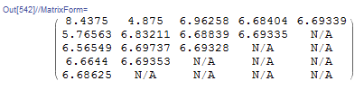
MATLAB files: File 1 (ex11_7.m) File 2 (trap_func.m)

RT4
The corresponding errors are given in the following table:
RT5

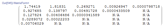
Comparing the table produced for the traditional trapezoidal method and that produced by the Romberg’s method reveals how powerful the Romberg’s method is. The Romberg table utilizes only the first 5 entries (up to $n=16$ ) in the traditional trapezoidal method table and then using a few calculations according to the Romberg’s method equation, produces a value with an absolute error of 0.0000799 which is less than that with traditional trapezoidal rule with $n=128$ .