Engineering at Alberta Courses » Bracketing Methods

Finding Roots of Equations: Bracketing Methods

An elementary observation from the previous method is that in most cases, the function changes signs around the roots of an equation. The bracketing methods rely on the intermediate value theorem.

4.2.1 Intermediate Value Theorem

Statement: Let $f:[a,b]\rightarrow \mathbb{R}$ be continuous and $f(a)\leq f(b)$ . Then, $\forall y\in[f(a),f(b)]:\exists x\in[a,b]$ such that $y=f(x)$ . The same applies if $f(b)\leq f(a)$ .
The proof for the intermediate value theorem relies on the assumption of continuity of the function $f$ . Intuitively, because the function $f$ is continuous, then for the values of $f$ to change from $f(a)$ to $f(b)$ it has to pass by every possible value between $f(a)$ and $f(b)$ . The consequence of the theorem is that if the function $f$ is such that $f(a)\leq 0 \leq f(b)$ , then, there is $x\in[a,b]$ such that $f(x)=0$ . We can proceed to find $x$ iteratively using either the bisection method or the false position method.

4.2.2 Bisection Method

In the bisection method, if $f(a)f(b)<0$ , an estimate for the root of the equation $f(x)=0$ can be found as the average of $a$ and $b$ :

$x_i=\frac{a+b}{2}$

Upon evaluating $f(x_i)$ , the next iteration would be to set either $a=x_i$ or $b=x_i$ such that for the next iteration the root $x_{i+1}$ is between $a$ and $b$ . The following describes an algorithm for the bisection method given $a<b$ , $f(x)$ , $\varepsilon_s$ , and maximum number of iterations:
Step 1: Evaluate $f(a)$ and $f(b)$ to ensure that $f(a)f(b)<0$ . Otherwise, exit with an error.
Step 2: Calculate the value of the root in iteration $i$ as $x_i=\frac{a_i+b_i}{2}$ . Check which of the following applies:

If $f(x_i)=0$ , then the root has been found, the value of the error $\varepsilon_r=0$ . Exit.
If $f(x_i)f(a_i)<0$ , then for the next iteration, $x_{i+1}$ is bracketed between $a_i$ and $x_i$ . The value of $\varepsilon_r=\frac{x_{i+1}-x_{i}}{x_{i+1}}$ .
If $f(x_i)f(b_i)<0$ , then for the next iteration, $x_{i+1}$ is bracketed between $x_i$ and $b_i$ . The value of $\varepsilon_r=\frac{x_{i+1}-x_{i}}{x_{i+1}}$ .

Step 3: Set $i=i+1$ . If $i$ reaches the maximum number of iterations or if $\varepsilon_r\leq \varepsilon_s$ , then the iterations are stopped. Otherwise, return to step 2 with the new interval $a_{i+1}$ and $b_{i+1}$ .

Example

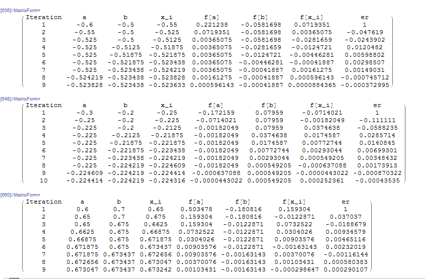
Setting $\varepsilon_s=0.0005$ and applying this process to $f(x)=\sin{5x}+\cos{2x}$ with $a=-0.6$ and $b=-0.5$ yields the estimate $x_9=-0.523633$ after 9 iterations with $\varepsilon_r=-0.000373$ as shown below. Similarly, applying this process to $f(x)=\sin{5x}+\cos{2x}$ with $a=-0.3$ and $b=-0.2$ yields the estimate $x_{10}=-0.224316$ after 10 iterations with $\varepsilon_r=-0.000435$ while applying this process to $f(x)=\sin{5x}+\cos{2x}$ with $a=0.6$ and $b=0.7$ yields the estimate $x_9=0.673242$ after 9 iterations with $\varepsilon_r=0.00029$ :

View Mathematica Code

Clear[f, x, ErrorTable, ei]
f[x_] := Sin[5 x] + Cos[2 x]
(*The following function returns x_i and the new interval (a,b) along with an error note. The order of the output is {xi,new a, new b, note}*)
bisec2[f_, a_, b_] := (xi = (a + b)/2; Which[
   f[a]*f[b] > 0, {xi, a, b, "Root Not Bracketed"},
   f[xi] == 0, {xi, a, b, "Root Found"},
   f[xi]*f[a] < 0, {xi, a, xi, "Root between a and xi"},
   f[xi]*f[b] < 0, {xi, xi, b, "Root between xi and b"}])

(*Problem Setup*)
MaxIter = 20;
eps = 0.0005;

(*First root*)
ErrorTable = {1};
ErrorNoteTable = {};
atable = {-0.6};
btable = {-0.5};
xtable = {};
i = 1;
Stopcode = "NoStopping";

While[And[i <= MaxIter, Stopcode == "NoStopping"],
 ri = bisec2[f, atable[[i]], btable[[i]]];
 If[ri[[4]] == "Root Not Bracketed", xtable = Append[xtable, ri[[1]]];ErrorNoteTable = Append[ErrorNoteTable, ri[[4]]]; Break[]];
 If[ri[[4]] == "Root Found", xtable = Append[xtable, ri[[1]]]; ErrorTable = Append[ErrorTable, 0];ErrorNoteTable = Append[ErrorNoteTable, ri[[4]]]; Break[]];
 atable = Append[atable, ri[[2]]];
 btable = Append[btable, ri[[3]]];
 xtable = Append[xtable, ri[[1]]];
 ErrorNoteTable = Append[ErrorNoteTable, ri[[4]]];
 If[i != 1,
  ei = (xtable[[i]] - xtable[[i - 1]])/xtable[[i]];
  ErrorTable = Append[ErrorTable, ei]];
 If[Abs[ErrorTable[[i]]] > eps, Stopcode = "NoStopping", Stopcode = "Stop"];
 i++]
Title = {"Iteration", "a", "b", "x_i", "f[a]", "f[b]", "f[x_i]", "er", "ErrorNote"};
T2 = Table[{i, atable[[i]], btable[[i]], xtable[[i]], f[atable[[i]]], f[btable[[i]]], f[xtable[[i]]], ErrorTable[[i]], ErrorNoteTable[[i]]}, {i, Length[xtable]}];
T2 = Prepend[T2, Title];
T2 // MatrixForm

(*Second Root*)
ErrorTable = {1};
ErrorNoteTable = {};
atable = {-0.3};
btable = {-0.2};
xtable = {};
i = 1;
Stopcode = "NoStopping";

While[And[i <= MaxIter, Stopcode == "NoStopping"],
 ri = bisec2[f, atable[[i]], btable[[i]]];
 If[ri[[4]] == "Root Not Bracketed", xtable = Append[xtable, ri[[1]]];ErrorNoteTable = Append[ErrorNoteTable, ri[[4]]]; Break[]];
 If[ri[[4]] == "Root Found", xtable = Append[xtable, ri[[1]]]; ErrorTable = Append[ErrorTable, 0];ErrorNoteTable = Append[ErrorNoteTable, ri[[4]]]; Break[]];
 atable = Append[atable, ri[[2]]];
 btable = Append[btable, ri[[3]]];
 xtable = Append[xtable, ri[[1]]];
 ErrorNoteTable = Append[ErrorNoteTable, ri[[4]]];
 If[i != 1,
  ei = (xtable[[i]] - xtable[[i - 1]])/xtable[[i]];
  ErrorTable = Append[ErrorTable, ei]];
 If[Abs[ErrorTable[[i]]] > eps, Stopcode = "NoStopping", Stopcode = "Stop"];
 i++]
Title = {"Iteration", "a", "b", "x_i", "f[a]", "f[b]", "f[x_i]", "er", "ErrorNote"};
T2 = Table[{i, atable[[i]], btable[[i]], xtable[[i]], f[atable[[i]]], f[btable[[i]]], f[xtable[[i]]], ErrorTable[[i]], ErrorNoteTable[[i]]}, {i, Length[xtable]}];
T2 = Prepend[T2, Title];
T2 // MatrixForm

(*Third Root*)
ErrorTable = {1};
ErrorNoteTable = {};
atable = {0.6};
btable = {0.7};
xtable = {};
i = 1;
Stopcode = "NoStopping";

While[And[i <= MaxIter, Stopcode == "NoStopping"],
 ri = bisec2[f, atable[[i]], btable[[i]]];
 If[ri[[4]] == "Root Not Bracketed", xtable = Append[xtable, ri[[1]]];ErrorNoteTable = Append[ErrorNoteTable, ri[[4]]]; Break[]];
 If[ri[[4]] == "Root Found", xtable = Append[xtable, ri[[1]]]; ErrorTable = Append[ErrorTable, 0];ErrorNoteTable = Append[ErrorNoteTable, ri[[4]]]; Break[]];
 atable = Append[atable, ri[[2]]];
 btable = Append[btable, ri[[3]]];
 xtable = Append[xtable, ri[[1]]];
 ErrorNoteTable = Append[ErrorNoteTable, ri[[4]]];
 If[i != 1,
  ei = (xtable[[i]] - xtable[[i - 1]])/xtable[[i]];
  ErrorTable = Append[ErrorTable, ei]];
 If[Abs[ErrorTable[[i]]] > eps, Stopcode = "NoStopping", Stopcode = "Stop"];
 i++]
Title = {"Iteration", "a", "b", "x_i", "f[a]", "f[b]", "f[x_i]", "er", "ErrorNote"};
T2 = Table[{i, atable[[i]], btable[[i]], xtable[[i]], f[atable[[i]]], f[btable[[i]]], f[xtable[[i]]], ErrorTable[[i]], ErrorNoteTable[[i]]}, {i, Length[xtable]}];
T2 = Prepend[T2, Title];
T2 // MatrixForm

View Python Code

import numpy as np
import pandas as pd

def f(x): return np.sin(5*x) + np.cos(2*x)
def bisec2(f,a,b):
  xi = (a + b)/2
  if f(a)*f(b) > 0: return [xi, a, b, "Root Not Bracketed"]
  elif f(xi) == 0: return [xi, a, b, "Root Found"]
  elif f(xi)*f(a) < 0: return [xi, a, xi, "Root between a and xi"]
  elif f(xi)*f(b) < 0: return [xi, xi, b, "Root between xi and b"]

def bisection(ErrorTable,ErrorNoteTable,atable,btable,xtable):
  MaxIter = 20
  eps = 0.0005
  Stopcode = "NoStopping"
  i = 0
  while i <= MaxIter and Stopcode == "NoStopping":
    ri = bisec2(f, atable[i], btable[i])
    if ri[3] == "Root Not Bracketed": 
      xtable.append(ri[0])
      ErrorNoteTable.append(ri[3])
      break
    if ri[3] == "Root Found":
      xtable.append(ri[0])
      ErrorTable.append(0)
      ErrorNoteTable.append(ri[3])
      break
    atable.append(ri[1])
    btable.append(ri[2])
    xtable.append(ri[0])
    ErrorNoteTable.append(ri[3])

    if i != 0:
      ei = (xtable[i] - xtable[i - 1])/xtable[i]
      ErrorTable.append(ei)
    if abs(ErrorTable[i]) > eps:
      Stopcode = "NoStopping"
    else:
      Stopcode = "Stop"
    i+=1
  T2 = ([[i, atable[i], btable[i], xtable[i], f(atable[i]), 
        f(btable[i]), f(xtable[i]), ErrorTable[i], 
        ErrorNoteTable[i]] for i in range(len(xtable))])
  T2 = pd.DataFrame(T2, columns=["Iteration", "a", "b", "x_i", "f[a]", "f[b]", "f[x_i]", "er", "ErrorNote"])
  display(T2)

# First Root
ErrorTable = [1]
ErrorNoteTable = []
atable = [-0.6]
btable = [-0.5]
xtable = []
print("First Root")
bisection(ErrorTable,ErrorNoteTable,atable,btable,xtable)

# Second Root
ErrorTable = [1]
ErrorNoteTable = []
atable = [-0.3]
btable = [-0.2]
xtable = []
print("Second Root")
bisection(ErrorTable,ErrorNoteTable,atable,btable,xtable)

# Third Root
ErrorTable = [1]
ErrorNoteTable = []
atable = [0.6]
btable = [0.7]
xtable = []
print("Third Root")
bisection(ErrorTable,ErrorNoteTable,atable,btable,xtable)

The following code can be used to implement the bisection method in MATLAB. For the sake of demonstration, it finds the roots of the function in above example. The example function is defined in another file

Download MATLAB file for the main script

Download MATLAB file for the example function

The following tool illustrates this process for $a=0.1$ and $b=0.9$ . Use the slider to view the process after each iteration. In the first iteration, the interval $[a,b]=[0.1,0.9]$ . $f(a)f(b)<0$ , so, $x_1=\frac{a+b}{2}=0.5$ . In the second iteration, the interval becomes $[0.5,0.9]$ and the new estimate $x_2=\frac{0.5+0.9}{2}=0.7$ . The relative approximate error in the estimate $\varepsilon_r=\frac{0.7-0.5}{0.7}=0.2857$ . You can view the process to see how it converges after 12 iterations.

Error Estimation

If $V_t$ is the true value of the root and $V_a$ is the estimate, then, the number of iterations $n$ needed to ensure that the absolute value of the error $|E|=|V_t-V_a|$ is less than or equal to a certain value can be easily obtained. Let $L=b-a$ be the length of the original interval used. The first estimate $x_1=\frac{a+b}{2}$ and so, in the next iteration, the interval where the root is contained has a length of $\frac{L}{2}$ . As the process evolves, the interval for the iteration number $n$ has a length of $\frac{L}{2^n}$ . Since the true value exists in an interval of length $\frac{L}{2^n}$ , the absolute value of the error is such that:

$|E|\leq \frac{L}{2^n}$

Therefore, for a desired estimate of the absolute value of the error, say $E_{max}$ , the number of iterations required is:

$\frac{L}{2^n}=E_{max}\Rightarrow n=\frac{\ln{\frac{L}{E_{max}}}}{\ln{2}}$

Example

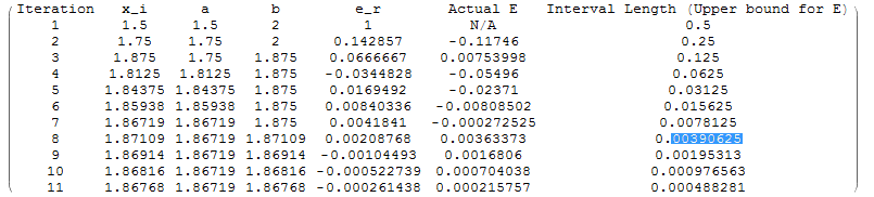
As an example, consider $f(x)=x^3+x^2-10$ , if we wish to find the root of the equation $f(x)=0$ in the interval $[1,2]$ with an absolute error less than or equal to 0.004, the number of iterations required is 8:

$n=\frac{\ln{\frac{1}{0.004}}}{\ln{2}}= 7.966 \approx 8$

The actual root with 10 significant digits is $V_t=1.867460025$ .
Using the process above, after the first iteration, $x_1=1.5$ and so, the root lies between $1.5$ and $2$ . So, the length of the interval is equal to 0.5 and the error in the estimate is less than 0.5. The length of the interval after iteration 8 is equal to 0.0039 and so the error in the estimate is less than 0.0039. It should be noted however that the actual error was less than this upper bound after the seventh iteration.

View Mathematica Code

Clear[f, x, tt, ErrorTable, nn];
f[x_] := x^3 + x^2 - 10;
bisec[f_, a_, b_] := (xi = (a + b)/2; 
   Which[f[a]*f[b] > 0, {xi, a, b, "Root Not Bracketed"}, 
    f[xi] == 0, {xi, a, b, "Root Found"}, 
    f[xi]*f[a] < 0, {xi, a, xi, "Root between a and xi"}, 
    f[xi]*f[b] < 0, {xi, xi, b, "Root between xi and b"}]);

(*Exact Solution*)
t = Solve[x^3 + x^2 - 10 == 0, x]
Vt = N[x /. t[[1]], 10]

(*Problem Setup*)
MaxIter = 20;
eps = 0.0005;

(*First root*)
x = {bisec[f, 1., 2]};
ErrorTable = {1};
ErrorTable2 = {"N/A"};
IntervalLength = {0.5};
i = 2;
While[And[i <= MaxIter, Abs[ErrorTable[[i - 1]]] > eps], 
 ri = bisec[f, x[[i - 1, 2]], x[[i - 1, 3]]];
 If[ri == "Error, root is not bracketed", 
  ErrorTable[[1]] = "Error, root is not bracketed"; Break[]];
 x = Append[x, ri]; ei = (x[[i, 1]] - x[[i - 1, 1]])/x[[i, 1]]; 
 e2i = x[[i, 1]] - Vt; ErrorTable = Append[ErrorTable, ei]; 
 IntervalLength = 
  Append[IntervalLength, (x[[i - 1, 3]] - x[[i - 1, 2]])/2]; 
 ErrorTable2 = Append[ErrorTable2, e2i]; i++]
x // MatrixForm
ErrorTable // MatrixForm
Title = {"Iteration", "x_i", "a", "b", "e_r", "Actual E", 
   "Interval Length (Upper bound for E)"};
T2 = Table[{i, x[[i, 1]], x[[i, 2]], x[[i, 3]], ErrorTable[[i]], 
    ErrorTable2[[i]], IntervalLength[[i]]}, {i, 1, Length[x]}];
T2 = Prepend[T2, Title];
T2 // MatrixForm

View Python Code

import sympy as sp
import pandas as pd

def f(x): return x**3 + x**2 - 10
def bisec(f,a,b):
  xi = (a + b)/2
  if f(a)*f(b) > 0: return [xi, a, b, "Root Not Bracketed"]
  elif f(xi) == 0: return [xi, a, b, "Root Found"]
  elif f(xi)*f(a) < 0: return [xi, a, xi, "Root between a and xi"]
  elif f(xi)*f(b) < 0: return [xi, xi, b, "Root between xi and b"]
    
# Exact Solution
x = sp.symbols('x')
t = list(sp.nonlinsolve([x**3 + x**2 - 10], [x]))
Vt = sp.N(t[0][0])
print("Vt:",Vt)

# Problem Setup
MaxIter = 20
eps = 0.0005

# First Root
x = [bisec(f, 1., 2)]
ErrorTable = [1]
ErrorTable2 = ["N/A"]
IntervalLength = [0.5]
i = 1

while i <= MaxIter and abs(ErrorTable[i - 1]) > eps:
  ri = bisec(f, x[i - 1][1], x[i - 1][2])
  if ri=="Error, root is not bracketed":
    ErrorTable[0]="Error, root is not bracketed"
    break
  x.append(ri)
  ei = (x[i][0] - x[i - 1][0])/x[i][0]
  e2i = x[i][0] - Vt
  ErrorTable.append(ei)
  IntervalLength.append((x[i - 1][2] - x[i - 1][1])/2)
  ErrorTable2.append(e2i)
  i+=1

print("x Table"); 
display(pd.DataFrame(x))
print("ErrorTable")
display(pd.DataFrame(ErrorTable))
T2 = ([[i, x[i][0], x[i][1], x[i][2], ErrorTable[i], ErrorTable2[i], 
      IntervalLength[i]] for i in range(len(x))])
pd.DataFrame(T2, columns=["Iteration", "x_i", "a", "b", "e_r", "Actual E", "Interval Length (Upper bound for E)"])

The procedure for solving the above example in MATLAB is available in the following files. The polynomial function is defined in a separate file.

Download MATLAB file for the main script

Download MATLAB file for the example polynomial function

4.2.3 False Position Method

In the false position method, the new estimate $x_i$ at iteration $i$ is obtained by considering the linear function passing through the two points $(a,f(a))$ and $(b,f(b))$ . The point of intersection of this line with the $x$ axis can be obtained using one of the following formulas:

$x_i=a-f(a)\frac{(b-a)}{f(b)-f(a)}=b-f(b)\frac{(b-a)}{f(b)-f(a)}=\frac{af(b)-bf(a)}{f(b)-f(a)}$

Upon evaluating $f(x_i)$ , the next iteration would be to set either $a=x_i$ or $b=x_i$ such that for the next iteration the root $x_{i+1}$ is between $a$ and $b$ . The following describes an algorithm for the false position method method given $a<b$ , $f(x)$ , $\varepsilon_s$ , and maximum number of iterations:
Step 1: Evaluate $f(a)$ and $f(b)$ to ensure that $f(a)f(b)<0$ . Otherwise exit with an error.
Step 2: Calculate the value of the root in iteration $i$ as $x_i=\frac{a_if(b_i)-bf(a_i)}{f(b_i)-f(a_i)}$ . Check which of the following applies:

If $f(x_i)=0$ , then the root has been found, the value of the error $\varepsilon_r=0$ . Exit.
If $f(x_i)f(a_i)<0$ , then for the next iteration, $x_{i+1}$ is bracketed between $a_i$ and $x_i$ . The value of $\varepsilon_r=\frac{x_{i+1}-x_{i}}{x_{i+1}}$ .
If $f(x_i)f(b_i)<0$ , then for the next iteration, $x_{i+1}$ is bracketed between $x_i$ and $b_i$ . The value of $\varepsilon_r=\frac{x_{i+1}-x_{i}}{x_{i+1}}$ .

Step 3: If $i$ reaches the maximum number of iterations or if $\varepsilon_r\leq \varepsilon_s$ , then the iterations are stopped. Otherwise, return to step 2.

Example

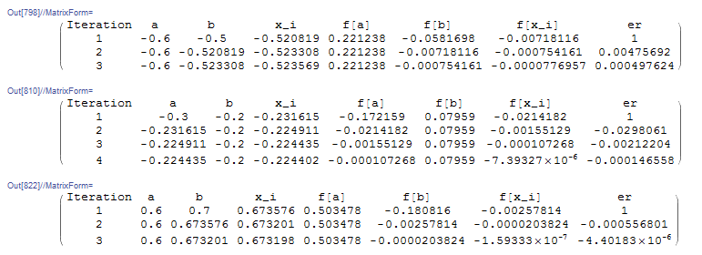
Setting $\varepsilon_s=0.0005$ and applying this process to $f(x)=\sin{5x}+\cos{2x}$ with $a=-0.6$ and $b=-0.5$ yields the estimate $x_3=-0.523569$ after 3 iterations with $\varepsilon_r=0.000498$ as shown below. Similarly, applying this process to $f(x)=\sin{5x}+\cos{2x}$ with $a=-0.3$ and $b=-0.2$ yields the estimate $x_4=-0.2244$ after 4 iterations with $\varepsilon_r=-0.00015$ while applying this process to $f(x)=\sin{5x}+\cos{2x}$ with $a=0.6$ and $b=0.7$ yields the estimate $x_3=0.673198$ after 3 iterations with $\varepsilon_r=-4.4\times 10^{-6}$ :

View Mathematica Code

Clear[f, x, ErrorTable, ei]
f[x_] := Sin[5 x] + Cos[2 x]
(*The following function returns x_i and the new interval (a,b) along with an error note. The order of the output is {xi,new a, new b, note}*)
falseposition[f_, a_, b_] := (xi = (a*f[b]-b*f[a])/(f[b]-f[a]); Which[
   f[a]*f[b] > 0, {xi, a, b, "Root Not Bracketed"},
   f[xi] == 0, {xi, a, b, "Root Found"},
   f[xi]*f[a] < 0, {xi, a, xi, "Root between a and xi"},
   f[xi]*f[b] < 0, {xi, xi, b, "Root between xi and b"}])

(*Problem Setup*)
MaxIter = 20;
eps = 0.0005;

(*First root*)
ErrorTable = {1};
ErrorNoteTable = {};
atable = {-0.6};
btable = {-0.5};
xtable = {};
i = 1;
Stopcode = "NoStopping";

While[And[i <= MaxIter, Stopcode == "NoStopping"],
 ri = falseposition[f, atable[[i]], btable[[i]]];
 If[ri[[4]] == "Root Not Bracketed", xtable = Append[xtable, ri[[1]]];ErrorNoteTable = Append[ErrorNoteTable, ri[[4]]]; Break[]];
 If[ri[[4]] == "Root Found", xtable = Append[xtable, ri[[1]]]; ErrorTable = Append[ErrorTable, 0];ErrorNoteTable = Append[ErrorNoteTable, ri[[4]]]; Break[]];
 atable = Append[atable, ri[[2]]];
 btable = Append[btable, ri[[3]]];
 xtable = Append[xtable, ri[[1]]];
 ErrorNoteTable = Append[ErrorNoteTable, ri[[4]]];
 If[i != 1,
  ei = (xtable[[i]] - xtable[[i - 1]])/xtable[[i]];
  ErrorTable = Append[ErrorTable, ei]];
 If[Abs[ErrorTable[[i]]] > eps, Stopcode = "NoStopping", Stopcode = "Stop"];
 i++]
Title = {"Iteration", "a", "b", "x_i", "f[a]", "f[b]", "f[x_i]", "er", "ErrorNote"};
T2 = Table[{i, atable[[i]], btable[[i]], xtable[[i]], f[atable[[i]]], f[btable[[i]]], f[xtable[[i]]], ErrorTable[[i]], ErrorNoteTable[[i]]}, {i, Length[xtable]}];
T2 = Prepend[T2, Title];
T2 // MatrixForm

(*Second Root*)
ErrorTable = {1};
ErrorNoteTable = {};
atable = {-0.3};
btable = {-0.2};
xtable = {};
i = 1;
Stopcode = "NoStopping";

While[And[i <= MaxIter, Stopcode == "NoStopping"],
 ri = falseposition[f, atable[[i]], btable[[i]]];
 If[ri[[4]] == "Root Not Bracketed", xtable = Append[xtable, ri[[1]]];ErrorNoteTable = Append[ErrorNoteTable, ri[[4]]]; Break[]];
 If[ri[[4]] == "Root Found", xtable = Append[xtable, ri[[1]]]; ErrorTable = Append[ErrorTable, 0];ErrorNoteTable = Append[ErrorNoteTable, ri[[4]]]; Break[]];
 atable = Append[atable, ri[[2]]];
 btable = Append[btable, ri[[3]]];
 xtable = Append[xtable, ri[[1]]];
 ErrorNoteTable = Append[ErrorNoteTable, ri[[4]]];
 If[i != 1,
  ei = (xtable[[i]] - xtable[[i - 1]])/xtable[[i]];
  ErrorTable = Append[ErrorTable, ei]];
 If[Abs[ErrorTable[[i]]] > eps, Stopcode = "NoStopping", Stopcode = "Stop"];
 i++]
Title = {"Iteration", "a", "b", "x_i", "f[a]", "f[b]", "f[x_i]", "er", "ErrorNote"};
T2 = Table[{i, atable[[i]], btable[[i]], xtable[[i]], f[atable[[i]]], f[btable[[i]]], f[xtable[[i]]], ErrorTable[[i]], ErrorNoteTable[[i]]}, {i, Length[xtable]}];
T2 = Prepend[T2, Title];
T2 // MatrixForm

(*Third Root*)
ErrorTable = {1};
ErrorNoteTable = {};
atable = {0.6};
btable = {0.7};
xtable = {};
i = 1;
Stopcode = "NoStopping";

While[And[i <= MaxIter, Stopcode == "NoStopping"],
 ri = falseposition[f, atable[[i]], btable[[i]]];
 If[ri[[4]] == "Root Not Bracketed", xtable = Append[xtable, ri[[1]]];ErrorNoteTable = Append[ErrorNoteTable, ri[[4]]]; Break[]];
 If[ri[[4]] == "Root Found", xtable = Append[xtable, ri[[1]]]; ErrorTable = Append[ErrorTable, 0];ErrorNoteTable = Append[ErrorNoteTable, ri[[4]]]; Break[]];
 atable = Append[atable, ri[[2]]];
 btable = Append[btable, ri[[3]]];
 xtable = Append[xtable, ri[[1]]];
 ErrorNoteTable = Append[ErrorNoteTable, ri[[4]]];
 If[i != 1,
  ei = (xtable[[i]] - xtable[[i - 1]])/xtable[[i]];
  ErrorTable = Append[ErrorTable, ei]];
 If[Abs[ErrorTable[[i]]] > eps, Stopcode = "NoStopping", Stopcode = "Stop"];
 i++]
Title = {"Iteration", "a", "b", "x_i", "f[a]", "f[b]", "f[x_i]", "er", "ErrorNote"};
T2 = Table[{i, atable[[i]], btable[[i]], xtable[[i]], f[atable[[i]]], f[btable[[i]]], f[xtable[[i]]], ErrorTable[[i]], ErrorNoteTable[[i]]}, {i, Length[xtable]}];
T2 = Prepend[T2, Title];
T2 // MatrixForm

View Python Code

import numpy as np
import pandas as pd

def f(x): return np.sin(5*x) + np.cos(2*x)
# The following function returns x_i and the new interval (a,b) along with an error note. The order of the output is {xi,new a, new b, note}
def falseposition(f,a,b):
  xi = (a*f(b)-b*f(a))/(f(b)-f(a))
  if f(a)*f(b) > 0: return [xi, a, b, "Root Not Bracketed"]
  elif f(xi) == 0: return [xi, a, b, "Root Found"]
  elif f(xi)*f(a) < 0: return [xi, a, xi, "Root between a and xi"]
  elif f(xi)*f(b) < 0: return [xi, xi, b, "Root between xi and b"]

def falseposition2(ErrorTable,ErrorNoteTable,atable,btable,xtable):
  MaxIter = 20
  eps = 0.0005
  Stopcode = "NoStopping"
  i = 0
  while i <= MaxIter and Stopcode == "NoStopping":
    ri = falseposition(f, atable[i], btable[i])
    if ri[3] == "Root Not Bracketed": 
      xtable.append(ri[0])
      ErrorNoteTable.append(ri[3])
      break
    if ri[3] == "Root Found":
      xtable.append(ri[0])
      ErrorTable.append(0)
      ErrorNoteTable.append(ri[3])
      break
    atable.append(ri[1])
    btable.append(ri[2])
    xtable.append(ri[0])
    ErrorNoteTable.append(ri[3])

    if i != 0:
      ei = (xtable[i] - xtable[i - 1])/xtable[i]
      ErrorTable.append(ei)
    if abs(ErrorTable[i]) > eps:
      Stopcode = "NoStopping"
    else:
      Stopcode = "Stop"
    i+=1
  T2 = ([[i, atable[i], btable[i], xtable[i], f(atable[i]), 
        f(btable[i]), f(xtable[i]), ErrorTable[i], 
        ErrorNoteTable[i]] for i in range(len(xtable))])
  T2 = pd.DataFrame(T2, columns=["Iteration", "a", "b", "x_i", "f[a]", "f[b]", "f[x_i]", "er", "ErrorNote"])
  display(T2)

# First Root
ErrorTable = [1]
ErrorNoteTable = []
atable = [-0.6]
btable = [-0.5]
xtable = []
print("First Root")
falseposition2(ErrorTable,ErrorNoteTable,atable,btable,xtable)

# Second Root
ErrorTable = [1]
ErrorNoteTable = []
atable = [-0.3]
btable = [-0.2]
xtable = []
print("Second Root")
falseposition2(ErrorTable,ErrorNoteTable,atable,btable,xtable)

# Third Root
ErrorTable = [1]
ErrorNoteTable = []
atable = [0.6]
btable = [0.7]
xtable = []
print("Third Root")
falseposition2(ErrorTable,ErrorNoteTable,atable,btable,xtable)

The procedure for implementing the false position root finding algorithm in MATLAB is available in the following files. The example function is defined in a separate file.

Download MATLAB file for the main script

Download MATLAB file for the example polynomial function

The following tool illustrates this process for $a=0.1$ and $b=0.9$ . Use the slider to view the process after each iteration. In the first iteration, the interval $[a,b]=[0.1,0.9]$ . $f(a)f(b)<0$ , so, $x_1=\frac{0.1f(0.9)-0.9f(0.1)}{f(0.9)-f(0.1)}=0.538249$ . In the second iteration, the interval becomes $[0.538249,0.9]$ and the new estimate $x_2=\frac{0.538249f(0.9)-0.9f(0.538249)}{f(0.9)-f(0.538249)}=0.693886$ . The relative approximate error in the estimate $\varepsilon_r=\frac{0.693886-0.538249}{0.693886}=0.224297$ . You can view the process to see how it converges after very few iterations.

4.2.4 Lecture video

4.2.5 Lecture video

Page Comments

Lucas Chin says:

December 10, 2024 at 1:33 am

Thank you so much for this content, this is very helpful, and will be passing this along to my classmates. I wish I could’ve found this earlier.

Reply
Samer Adeeb says:

December 10, 2024 at 7:12 am

Thank you

Reply

Open Educational Resources

Finding Roots of Equations: Bracketing Methods

4.2.1 Intermediate Value Theorem

4.2.2 Bisection Method

Example

Error Estimation

Example

4.2.3 False Position Method

Example

4.2.4 Lecture video

4.2.5 Lecture video

Page Comments

Leave a Reply Cancel reply