
Curve Fitting: Linear Regression
Linear Regression
Given a set of data  with
with  , a linear model fit to this set of data has the form:
![\[y(x)=ax+b\]](https://engcourses-uofa.ca/wp-content/ql-cache/quicklatex.com-a774144ced173f2e7ef0299095d10766_l3.png "Rendered by QuickLaTeX.com")
where  and
and  are the model parameters. The model parameters can be found by minimizing the sum of the squares of the difference (
 ) between the data points and the model predictions:
![\[S=\sum_{i=1}^n\left(y(x_i)-y_i\right)^2\]](https://engcourses-uofa.ca/wp-content/ql-cache/quicklatex.com-5ff51969f2f627d835a000a989bf0780_l3.png "Rendered by QuickLaTeX.com")
Substituting for  yields:
![\[S=\sum_{i=1}^n\left(ax_i+b-y_i\right)^2\]](https://engcourses-uofa.ca/wp-content/ql-cache/quicklatex.com-d7b533248f47153fbe28e10e8149df36_l3.png "Rendered by QuickLaTeX.com")
In order to minimize , we need to differentiate with respect to the unknown parameters and and set these two equations to zero:
![\[\begin{split}\frac{\partial S}{\partial a}&=2\sum_{i=1}^n\left(\left(ax_i+b-y_i\right)x_i\right)=0\\\frac{\partial S}{\partial b}&=2\sum_{i=1}^n\left(ax_i+b-y_i\right)=0\\\end{split}\]](https://engcourses-uofa.ca/wp-content/ql-cache/quicklatex.com-b65279d1c7a68f8d6c44a06acdac85af_l3.png "Rendered by QuickLaTeX.com")
Solving the above two equations yields the best linear fit to the data. The solution for and has the form:
![\[\begin{split}a&=\frac{n\sum_{i=1}^nx_iy_i-\sum_{i=1}^nx_i\sum_{i=1}^ny_i}{n\sum_{i=1}^nx_i^2-\left(\sum_{i=1}^nx_i\right)^2}\\b&=\frac{\sum_{i=1}^ny_i-a\sum_{i=1}^nx_i}{n}\end{split}\]](https://engcourses-uofa.ca/wp-content/ql-cache/quicklatex.com-14fb4c30a307d0bf9b199a60a2e0e149_l3.png "Rendered by QuickLaTeX.com")
The built-in function “Fit” in mathematica can be used to find the best linear fit to any data. The following code illustrates the procedure to use “Fit” to find the equation of the line that fits the given array of data:
View Mathematica CodeData = {{1, 0.5}, {2, 2.5}, {3, 2}, {4, 4.0}, {5, 3.5}, {6, 6.0}, {7, 5.5}};
y = Fit[Data, {1, x}, x]
Plot[y, {x, 1, 7}, Epilog -> {PointSize[Large], Point[Data]}, AxesLabel -> {"x", "y"}, AxesOrigin -> {0, 0}]
import numpy as np
import matplotlib.pyplot as plt

Data = [[1, 0.5], [2, 2.5], [3, 2], [4, 4.0], [5, 3.5], [6, 6.0], [7,  5.5]]
p = np.polyfit([point[0] for point in Data],
               [point[1] for point in Data], 1)
x = np.linspace(1, 7)
y = np.poly1d(p)
plt.plot(x, y(x))
plt.title(y)
plt.scatter([point[0] for point in Data],[point[1] for point in Data], c='k')
plt.xlabel("x"); plt.ylabel("y")
plt.grid(); plt.show()
Coefficient of Determination
The coefficient of determination, denoted  or
or  and pronounced
  squared, is a number that provides a statistical measure of how the produced model fits the data. The value of can be calculated as follows:
![\[ R^2=1-\frac{\sum_{i=1}^n\left(y_i-y(x_i)\right)^2}{\sum_{i=1}^n\left(y_i-\frac{1}{n}\sum_{i=1}^ny_i\right)^2}\]](https://engcourses-uofa.ca/wp-content/ql-cache/quicklatex.com-3acc0773657b551ed19f8fc5f6ed4207_l3.png "Rendered by QuickLaTeX.com")
The equation above implies that  . A value closer to 1 indicates that the model is a good fit for the data while a value of 0 indicates that the model does not fit the data.
Using Mathematica and/or Excel
The built-in Mathematica function “LinearModelFit” provides the statistical measures associated with a linear regression model, including the confidence intervals in the parameters and . However, these are not covered in this course. The “LinearModelFit” can be used to output the of the linear fit as follows:
Data = {{1, 0.5}, {2, 2.5}, {3, 2}, {4, 4.0}, {5, 3.5}, {6, 6.0}, {7, 5.5}};
y2 = LinearModelFit[Data, x, x]
y = Normal[y2]
y3 = y2["RSquared"]
Plot[y, {x, 1, 7}, Epilog -> {PointSize[Large], Point[Data]}, AxesLabel -> {"x", "y"}, AxesOrigin -> {0, 0}]
import numpy as np
from scipy import stats
import matplotlib.pyplot as plt

Data = [[1, 0.5], [2, 2.5], [3, 2], [4, 4.0], [5, 3.5], [6, 6.0], [7,  5.5]]
p = np.polyfit([point[0] for point in Data],
               [point[1] for point in Data], 1)
print("p: ",p)
slope, intercept, r_value, p_value, std_err = stats.linregress([point[0] for point in Data],
                                                               [point[1] for point in Data])
print("R Squared: ",r_value**2)
y = np.poly1d(p)
print("y:",y)
x = np.linspace(1, 7)
plt.title(y)
plt.plot(x, y(x))
plt.scatter([point[0] for point in Data],[point[1] for point in Data], c='k')
plt.xlabel("x"); plt.ylabel("y")
plt.grid(); plt.show()
The following user-defined Mathematica procedure finds the linear fit and and draws the curve for a set of data:
Clear[a, b, x]
Data = {{1, 0.5}, {2, 2.5}, {3, 2}, {4, 4.0}, {5, 3.5}, {6, 6.0}, {7, 5.5}};
LinearFit[Data_] :=
 (n = Length[Data];
  a = (n*Sum[Data[[i, 1]]*Data[[i, 2]], {i, 1, n}] - Sum[Data[[i, 1]], {i, 1, n}]*Sum[Data[[i, 2]], {i, 1, n}])/(n*Sum[Data[[i, 1]]^2, {i, 1, n}] - (Sum[Data[[i, 1]], {i, 1, n}])^2);
  b=(Sum[Data[[i, 2]], {i, 1, n}] - a*Sum[Data[[i, 1]], {i, 1, n}])/    n;
   RSquared=1-Sum[(Data[[i,2]]-a*Data[[i,1]]-b)^2,{i,1,n}]/Sum[(Data[[i,2]]-1/n*Sum[Data[[j,2]],{j,1,n}])^2,{i,1,n}];
  {RSquared,a,b })
LinearFit[Data]
RSquared=LinearFit[Data][[1]]
a = LinearFit[Data][[2]]
b = LinearFit[Data][[3]]
y = a*x + b;
Plot[y, {x, 1, 7}, Epilog -> {PointSize[Large], Point[Data]}, AxesLabel -> {"x", "y"}, AxesOrigin -> {0, 0} ]
import numpy as np
import matplotlib.pyplot as plt

Data = [[1, 0.5], [2, 2.5], [3, 2], [4, 4.0], [5, 3.5], [6, 6.0], [7, 5.5]]
def LinearFit(Data):
  n = len(Data)
  a = (n*sum([Data[i][0]*Data[i][1] for i in range(n)]) - sum([Data[i][0] for i in range(n)])*sum([Data[i][1] for i in range(n)]))/(n*sum([Data[i][0]**2 for i in range(n)]) - sum([Data[i][0] for i in range(n)])**2)
  b = (sum([Data[i][1] for i in range(n)]) - a*sum([Data[i][0] for i in range(n)]))/n
  RSquared = 1 - sum([(Data[i][1] - a*Data[i][0] - b)**2 for i in range(n)])/sum([(Data[i][1] - 1/n*sum([Data[j][1] for j in range(n)]))**2 for i in range(n)])
  return [RSquared, a, b]
x = np.linspace(0,7)
LinearFit(Data)
print("LinearFit(Data): ",LinearFit(Data))
RSquared = LinearFit(Data)[0]
print("RSquared: ",RSquared)
a = LinearFit(Data)[1]
b = LinearFit(Data)[2]
print("a: ",a)
print("b: ",b)
y = a*x + b;
plt.plot(x, y)
plt.scatter([point[0] for point in Data],[point[1] for point in Data], c='k')
plt.xlabel("x"); plt.ylabel("y")
plt.grid(); plt.show()
Microsoft Excel can be used to provide the linear fit (linear regression) for any set of data. First, the curve is plotted using “XY scatter”. Afterwards, right clicking on the data curve and selecting “Add Trendline” will provide the linear fit. You can format the trendline to “show equation on chart” and .
Example
Find the best linear fit to the data (1,0.5), (2,2.5), (3,2), (4,4), (5,3.5), (6,6), (7,5.5).
Solution
Using the equations for , , and :
![\[\begin{split}a&=\frac{n\sum_{i=1}^nx_iy_i-\sum_{i=1}^nx_i\sum_{i=1}^ny_i}{n\sum_{i=1}^nx_i^2-\left(\sum_{i=1}^nx_i\right)^2}=\frac{7(119.5)-(28)(24)}{7(140)-(28)^2}=0.839286\\b&=\frac{\sum_{i=1}^ny_i-a\sum_{i=1}^nx_i}{n}=\frac{24-(0.839286)(28)}{7}=0.071429\\R^2&=1-\frac{\sum_{i=1}^n\left(y_i-y(x_i)\right)^2}{\sum_{i=1}^n\left(y_i-\frac{1}{n}\sum_{i=1}^ny_i\right)^2}=1-\frac{2.9911}{22.7143}=0.8683\end{split}\]](https://engcourses-uofa.ca/wp-content/ql-cache/quicklatex.com-f2ea247688483c9eadf1133bc4a0240e_l3.png "Rendered by QuickLaTeX.com")
Microsoft Excel can easily be used to generate the values for , , and as shown in the following sheet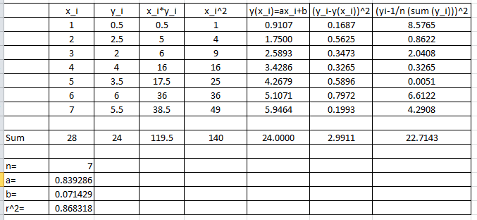
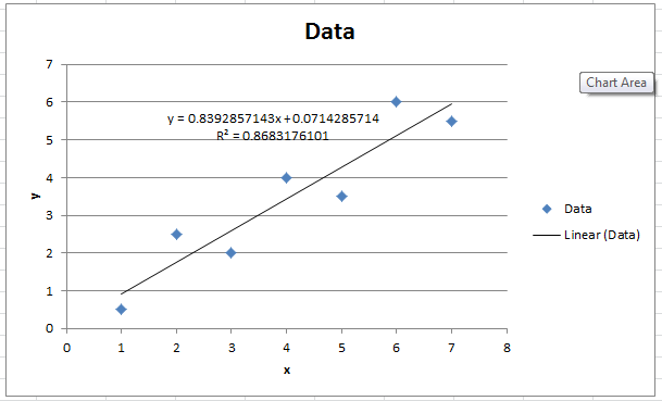
The following is the Microsoft Excel chart produced as described above.
You can upload some data on the online Python app on mecsimcalc that performs these calculations which is embedded below as well.
The following link provides the MATLAB code for implementing the linear curve fit.