
Solution Methods for IVPs: (Explicit) Euler Method
(Explicit) Euler Method
The Euler method is one of the simplest methods for solving first-order IVPs. Consider the following IVP:
![\[\frac{\mathrm{d}x}{\mathrm{d}t}=F(x,t)\]](https://engcourses-uofa.ca/wp-content/ql-cache/quicklatex.com-6944c0bf340e6c84565355872b70290a_l3.png "Rendered by QuickLaTeX.com")
Assuming that the value of the dependent variable
 (say
(say  ) is known at an initial value
  , then, we can use a Taylor approximation to estimate the value of at
  , namely
  with
with  :
: ![\[x(t_{i+1})=x_i+\frac{\mathrm{d}x}{\mathrm{d}t}\bigg|_{t_i} (h) +\mathcal{O}(h^2)\]](https://engcourses-uofa.ca/wp-content/ql-cache/quicklatex.com-41745a8fa1160b7363109e9aac454e62_l3.png "Rendered by QuickLaTeX.com")
Substituting the differential equation into the above equation yields:
![\[x(t_{i+1})=x_i+F(x_i,t_i) (h) +\mathcal{O}(h^2)\]](https://engcourses-uofa.ca/wp-content/ql-cache/quicklatex.com-9749135953d0fd446d534737c2727844_l3.png "Rendered by QuickLaTeX.com")
Therefore, as an approximation, an estimate for
can be taken as  as follows:
 ![\[x(t_{i+1})\approx x_{i+1}=x_i+F(x_i,t_i) (h)\]](https://engcourses-uofa.ca/wp-content/ql-cache/quicklatex.com-a77eb8dbe87a9166b437945caafd4f8d_l3.png "Rendered by QuickLaTeX.com")
Using this estimate, the local truncation error is thus proportional to the square of the step size with the constant of proportionality related to the second derivative of
, which is the first derivative of the given IVP: ![\[E_{\mbox{local}}=\mathcal{O}(h^2)\]](https://engcourses-uofa.ca/wp-content/ql-cache/quicklatex.com-2cee0f744ce6edc64ca4c6bb72af5ca5_l3.png "Rendered by QuickLaTeX.com")
If the errors from each interval are added together, with
 being the number of intervals and
  the total length
  , then, the total error is:
 ![\[E=\mathcal{O}(h^2) \frac{L}{h}=\mathcal{O}(h)\]](https://engcourses-uofa.ca/wp-content/ql-cache/quicklatex.com-1069b99640fa20c52fbb1fe77e96dca7_l3.png "Rendered by QuickLaTeX.com")
There are many examples in engineering and biology in which such IVPs appear. Check this page for examples.
The following Mathematica code provides a procedure whose inputs are
- The differential equation as a function of the dependent variable and the independent variable
 .
. - The step size
 .
. - The initial value
 and the final value
  of the independent variable.
 - The initial value
 .
.
The procedure then carries on the Euler method and outputs the required data vector.
View Mathematica CodeEulerMethod[fp_, x0_, h_, t0_, tmax_] :=
(n = (tmax - t0)/h + 1;
xtable = Table[0, {i, 1, n}];
xtable[[1]] = x0;
Do[xtable[[i]] = xtable[[i - 1]] + h*fp[xtable[[i - 1]], t0 + (i - 2) h], {i, 2, n}];
Data = Table[{t0 + (i - 1)*h, xtable[[i]]}, {i, 1, n}];
Data)
function1[y_, t_] := 0.05 y
function2[x_, t_] := 0.015 x
EulerMethod[function1, 35, 1.0, 0, 50] // MatrixForm
EulerMethod[function2, 35, 1.0, 0, 50] // MatrixForm
def EulerMethod(fp, x0, h, t0, tmax):
  n = int((tmax - t0)/h + 1)
  xtable = [0 for i in range(n)]
  xtable[0] = x0
  for i in range(1,n):
    xtable[i] = xtable[i - 1] + h*fp(xtable[i - 1], t0 + (i - 1)*h)
  Data = [[t0 + i*h, xtable[i]] for i in range(n)]
  return Data
def function1(y, t): return 0.05*y
def function2(x, t): return 0.015*x
display(EulerMethod(function1, 35, 1.0, 0, 50))
display(EulerMethod(function2, 35, 1.0, 0, 50))
Example 1
The Canadian population at  (current year) is 35 million. If 2.5% of the population have a child in a given year, while the death rate is 1% of the population, what will the population be in 50 years? What if 6% of the population have a child in a given year and the death rate is kept constant at 1%, what will the population be in 50 years?
Solution
The rate of growth is directly proportional to the current population with the constant of proportionality  . If represents the population in millions and represents the time in years, then the IVP is given by:
![\[\frac{\mathrm{d}x}{\mathrm{d}t}=0.015 x\]](https://engcourses-uofa.ca/wp-content/ql-cache/quicklatex.com-c6e2b43da9719e04ae6845d61d78b4dc_l3.png "Rendered by QuickLaTeX.com")
With the initial condition of
 , the exact solution to this differential equation is:
 ![\[x=35e^{0.015t}\]](https://engcourses-uofa.ca/wp-content/ql-cache/quicklatex.com-3448591a3ed00b6f197beea87811f9ed_l3.png "Rendered by QuickLaTeX.com")
If the birth rate is 6%, then
 and the exact solution of the population follows the following equation:
 ![\[x=35e^{0.05t}\]](https://engcourses-uofa.ca/wp-content/ql-cache/quicklatex.com-d07506010121b816767788e9ee490601_l3.png "Rendered by QuickLaTeX.com")
The Euler method provides a numerical solution as follows. Using a step size of  , we can set
  years. The value of
  is given as 35 million. When
  , the value of
  in millions is given by:
![\[x_1=x_0+h\frac{\mathrm{d}x}{\mathrm{d}t}\bigg|_{x=x_0,t=t_0}=35+0.015\times 35=35.525\]](https://engcourses-uofa.ca/wp-content/ql-cache/quicklatex.com-5c0d8eb3bcdb4f07ecd68e52a063f01e_l3.png "Rendered by QuickLaTeX.com")
The value of
 is given by:
 ![\[x_2=x_1+h\frac{\mathrm{d}x}{\mathrm{d}t}\bigg|_{x=x_1,t=t_1}=35.525+0.015\times 35.525=36.0579\]](https://engcourses-uofa.ca/wp-content/ql-cache/quicklatex.com-f3759c02571f5e089f2acee6fcf5d8fc_l3.png "Rendered by QuickLaTeX.com")
Iterating further, the values of
at each time point can be obtained. The following is the Microsoft Excel table showing the values of in years and the corresponding values of the population in millions: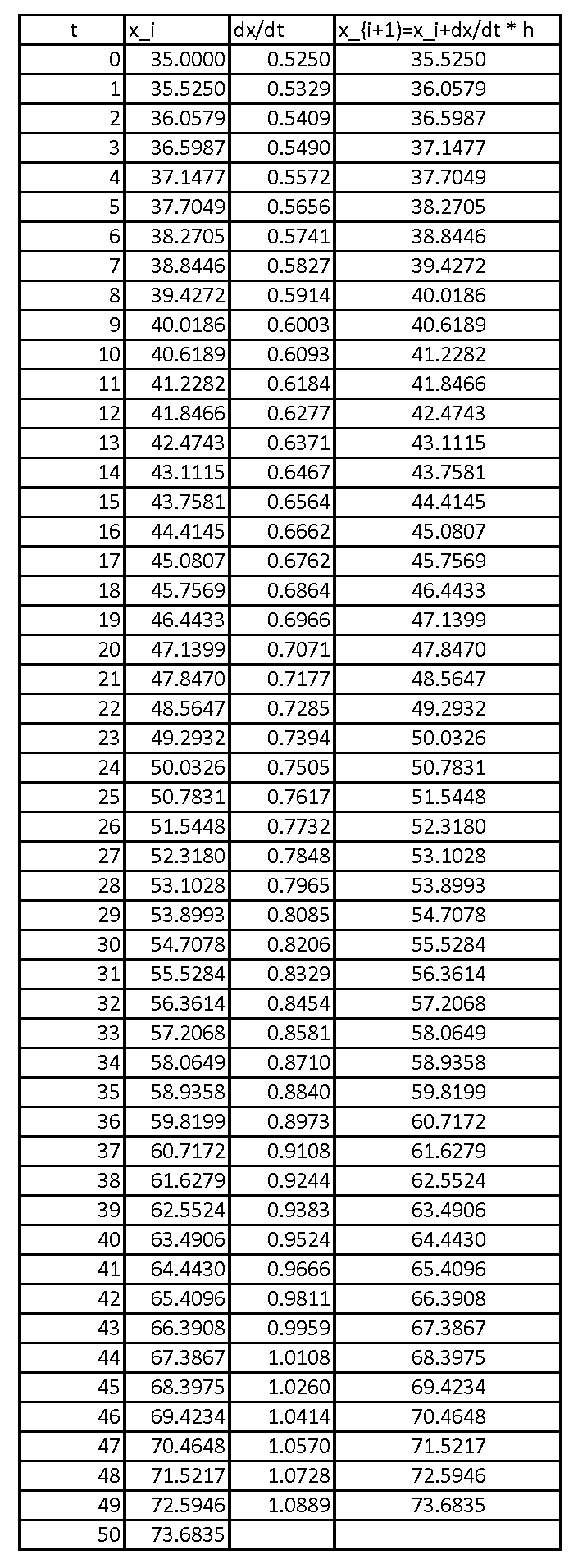
When
, the numerical procedure produces a very good approximation for the population at  years. The error between the prediction of the exact solution to the differential equation and the numerical value at is given in millions by:
 ![\[E=35e^{(0.015\times 50)} - 73.6835=74.095-73.6835=0.4\]](https://engcourses-uofa.ca/wp-content/ql-cache/quicklatex.com-d1a61f7bd3d159d0bab072c0bde1047b_l3.png "Rendered by QuickLaTeX.com")
The relative error in this case is given by:
![\[E_r=\frac{0.4}{74.095}=0.005\]](https://engcourses-uofa.ca/wp-content/ql-cache/quicklatex.com-fbb86d9702f24f8917aa56869ff01cf2_l3.png "Rendered by QuickLaTeX.com")
For the second case, when  , the value of in millions is given by:
![\[x_1=x_0+h\frac{\mathrm{d}x}{\mathrm{d}t}\bigg|_{x=x_0,t=t_0}=35+0.05\times 35=36.75\]](https://engcourses-uofa.ca/wp-content/ql-cache/quicklatex.com-3afeeec18b4eda3bbe38b496c7fee18e_l3.png "Rendered by QuickLaTeX.com")
Proceeding iteratively, the following is the Microsoft Excel table showing the values of
in years and the corresponding values of the population in millions: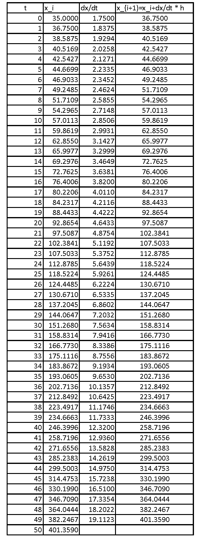
Compared to the previous case, when
, the numerical procedure is not as good. The error between the prediction of the exact solution to the differential equation and the numerical value at is given in millions by: ![\[E=35e^{(0.05\times 50)} - 401.359=426.387-401.359=25.0283\]](https://engcourses-uofa.ca/wp-content/ql-cache/quicklatex.com-372d4e2bd033b5195ad421ef66ff725b_l3.png "Rendered by QuickLaTeX.com")
The relative error in this case is given by:
![\[E_r=\frac{25.0283}{426.387}=0.06\]](https://engcourses-uofa.ca/wp-content/ql-cache/quicklatex.com-21f9d6ef23d4ca18fc659a213c0220fa_l3.png "Rendered by QuickLaTeX.com")
The following is the graph showing the exact solution versus the data using the Euler method for both cases. The Mathematica code used is given below. Notice how the error in the Euler method increases as
increases.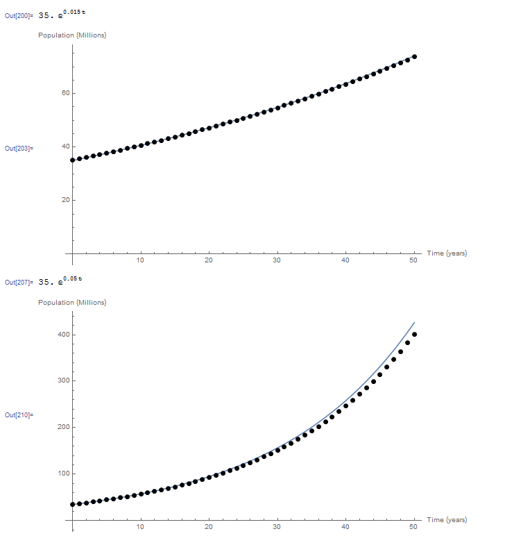 View Mathematica Code
EulerMethod[fp_, x0_, h_, t0_, tmax_] :=
  (n = (tmax - t0)/h + 1;
  xtable = Table[0, {i, 1, n}];
  xtable[[1]] = x0;
  Do[xtable[[i]] =  xtable[[i - 1]] + h*fp[xtable[[i - 1]], t0 + (i - 2) h], {i, 2, n}];
  Data = Table[{t0 + (i - 1)*h, xtable[[i]]}, {i, 1, n}];
  Data)

Clear[x, xtable]
k = 0.015;
a = DSolve[{x'[t] == k*x[t], x[0] == 35}, x, t];
x = x[t] /. a[[1]]
fp[x_, t_] := k*x;
Data = EulerMethod[fp, 35, 1.0, 0, 50];
Plot[x, {t, 0, 50}, Epilog -> {PointSize[Large], Point[Data]}, AxesOrigin -> {0, 0}, AxesLabel -> {"Time (years)", "Population (Millions)"}]

Clear[x, xtable]
k = 0.05;
a = DSolve[{x'[t] == k*x[t], x[0] == 35}, x, t];
x = x[t] /. a[[1]]
fp[x_, t_] := k*x;
Data = EulerMethod[fp, 35, 1.0, 0, 50];
Plot[x, {t, 0, 50}, Epilog -> {PointSize[Large], Point[Data]}, AxesOrigin -> {0, 0}, AxesLabel -> {"Time (years)", "Population (Millions)"}]
# UPGRADE: need Sympy 1.2 or later, upgrade by running: "!pip install sympy --upgrade" in a code cell
# !pip install sympy --upgrade
import numpy as np
import sympy as sp
import matplotlib.pyplot as plt
sp.init_printing(use_latex=True)

def EulerMethod(fp, x0, h, t0, tmax):
  n = int((tmax - t0)/h + 1)
  xtable = [0 for i in range(n)]
  xtable[0] = x0
  for i in range(1,n):
    xtable[i] = xtable[i - 1] + h*fp(xtable[i - 1], t0 + (i - 1)*h)
  Data = [[t0 + i*h, xtable[i]] for i in range(n)]
  return Data

x = sp.Function('x')
t = sp.symbols('t')
k = 0.015
sol = sp.dsolve(x(t).diff(t) - k*x(t), ics={x(0): 35})
display(sol)
def fp(x, t): return k*x
Data = EulerMethod(fp, 35, 1.0, 0, 50)
x_val = np.arange(0,50,0.1)
plt.plot(x_val, [sol.subs(t, i).rhs for i in x_val])
plt.scatter([point[0] for point in Data],[point[1] for point in Data])
plt.xlabel("Time (years)"); plt.ylabel("Population (Millions)")
plt.grid(); plt.show()

k = 0.05
sol = sp.dsolve(x(t).diff(t) - k*x(t), ics={x(0): 35})
display(sol)
Data = EulerMethod(fp, 35, 1.0, 0, 50)
plt.plot(x_val, [sol.subs(t, i).rhs for i in x_val])
plt.scatter([point[0] for point in Data],[point[1] for point in Data])
plt.xlabel("Time (years)"); plt.ylabel("Population (Millions)")
plt.grid(); plt.show()
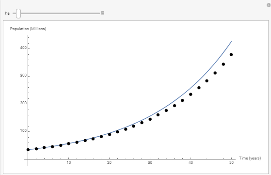
The following tool illustrates the effect of choosing the step size on the difference between the numerical solution (shown as dots) and the exact solution (shown as the blue curve) for the case when . The smaller the step size, the more accurate the solution is. The higher the value of , the more the numerical solution deviates from the exact solution. The error increases away from the initial conditions.
Example 2
This example is adopted from this page. A lake of volume  has an initial concentration of a particular pollutant of
  parts per billion (ppb). This pollutant is due to a pesticide that is no longer available in the market. The volume of the lake is constant throughout the year, with daily water flowing into and out of the lake at the rate of
  . As the pesticide is no longer used, the concentration of the pollutant in the surrounding soil is given in ppb as a function of (days) by
  which indicates that the concentration is following an exponential decay. This concentration can be assumed to be that of the pollutant in the fluid flowing into the lake. The concentration of the pollutant in the fluid flowing out of the lake is the same as the concentration in the lake. What is the concentration of this particular pollutant in the lake after two years?
Solution
The first step in this problem is to properly write the differential equation that needs to be solved. If  is the total amount of pollutant in the lake, then, the rate of change of with respect to is equal to the total amount of pollutant entering into the lake per day. Each day, the total amount of pollutant entering the lake is given by
  , while the total amount of pollutant exiting the lake is given by
  , where
  is the concentration of the pollutant in the lake. Therefore:
![\[\frac{\mathrm{d}\alpha}{\mathrm{d}t}=\left(100+50\cos{(2\pi t/365)}\right)\left(c_{in}-c\right)\]](https://engcourses-uofa.ca/wp-content/ql-cache/quicklatex.com-7064a92eb828396d1fdd4f91a47e3d77_l3.png "Rendered by QuickLaTeX.com")
The concentration is equal to the total amount divided by the volume of the lake, therefore, the differential equation in terms of
is given by: ![\[\frac{\mathrm{d}c}{\mathrm{d}t}=\frac{\left(100+50\cos{(2\pi t/365)}\right)}{10000}\left(c_{in}-c\right)=\frac{\left(100+50\cos{(2\pi t/365)}\right)}{10000}\left(5e^{\left(\frac{-2t}{1000}\right)}-c\right)\]](https://engcourses-uofa.ca/wp-content/ql-cache/quicklatex.com-6efc9019aafeb6142b9d1792256bcf56_l3.png "Rendered by QuickLaTeX.com")
Notice that finding an exact solution to the above differential equation is not an easy task and a numerical solution would be the preferred solution in this case. Taking
day,  , and
, and  ppb the Euler method can be used to find the concentration at
  days. You can download the Microsoft Excel file example2.xlsx showing the calculations and the produced graph.
Taking
 day, we will show the calculations for the estimates
  and
and  . At
. At  day:
day: ![\[\begin{split}c_1&=c_0+h\frac{\mathrm{d}c}{\mathrm{d}t}\bigg|_{c=c_0,t=t_0}\\&=5+1\left(\frac{\left(100+50\cos{(2\pi 0/365)}\right)}{10000}\left(5e^{\left(\frac{-2(0)}{1000}\right)}-5\right)\right)\\&=5\end{split}\]](https://engcourses-uofa.ca/wp-content/ql-cache/quicklatex.com-d6c544bc0a804273304a2b821c1f1bef_l3.png "Rendered by QuickLaTeX.com")
At
 days:
days: ![\[\begin{split}c_2&=c_1+h\frac{\mathrm{d}c}{\mathrm{d}t}\bigg|_{c=c_1,t=t_1}\\&=5+1\left(\frac{\left(100+50\cos{(2\pi 1/365)}\right)}{10000}\left(5e^{\left(\frac{-2(1)}{1000}\right)}-5\right)\right)\\&=4.9999\end{split}\]](https://engcourses-uofa.ca/wp-content/ql-cache/quicklatex.com-16b9a591aeda22fe068603460cf4f9af_l3.png "Rendered by QuickLaTeX.com")
Carrying on produces the values of
at the remaining time intervals up to  days. The following is the output produced by the Mathematica code below.
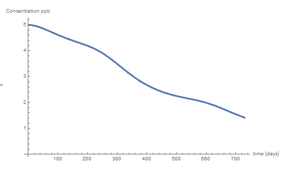 View Mathematica Code
EulerMethod[fp_, x0_, h_, t0_, tmax_] :=
 (n = (tmax - t0)/h + 1;
  xtable = Table[0, {i, 1, n}];
  xtable[[1]] = x0;
  Do[xtable[[i]] =  xtable[[i - 1]] + h*fp[xtable[[i - 1]], t0 + (i - 2) h], {i, 2, n}];
  Data = Table[{t0 + (i - 1)*h, xtable[[i]]}, {i, 1, n}];
  Data)
f[t_] := 100 + 50*Cos[2 Pi*t/365];
cin[t_] := 5 E^(-2 t/1000);
fp[c_, t_] := f[t] (cin[t] - c)/10000;
Data = EulerMethod[fp, 5, 1.0, 0, 365*2];
ListPlot[Data, AxesLabel -> {"time (days)", "Concentration ppb"}]
import numpy as np
import matplotlib.pyplot as plt

def EulerMethod(fp, x0, h, t0, tmax):
  n = int((tmax - t0)/h + 1)
  xtable = [0 for i in range(n)]
  xtable[0] = x0
  for i in range(1,n):
    xtable[i] = xtable[i - 1] + h*fp(xtable[i - 1], t0 + (i - 1)*h)
  Data = [[t0 + i*h, xtable[i]] for i in range(n)]
  return Data
def f(t): return 100 + 50*np.cos(2*np.pi*t/365)
def cin(t): return 5*np.exp(-2*t/1000)
def fp(c, t): return f(t)*(cin(t) - c)/10000
Data = EulerMethod(fp, 5, 1.0, 0, 365*2)
plt.scatter([point[0] for point in Data],[point[1] for point in Data])
plt.xlabel("Time (days)"); plt.ylabel("Concentration ppb")
plt.grid(); plt.show()
Example 3
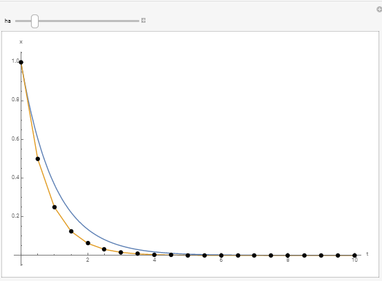
In this example we investigate the issue of stability of numerical solution of differential equations using the Euler method. Consider the IVP of the form:
![\[\frac{\mathrm{d}x}{\mathrm{d}t}=-x\]](https://engcourses-uofa.ca/wp-content/ql-cache/quicklatex.com-44b5815cfef286d7eca63da9db0ec821_l3.png "Rendered by QuickLaTeX.com")
If
 , compare the two solutions taking a step size of
  , and a step size of
  .
.
Solution
The exact solution to the given equation is given by:
![\[x=e^{-t}\]](https://engcourses-uofa.ca/wp-content/ql-cache/quicklatex.com-0723d0c9e4236f51da3a921e4d8b07a4_l3.png "Rendered by QuickLaTeX.com")
Using an explicit Euler scheme, the value of
can be obtained as follows: ![\[x_{i+1}=x_i+h\frac{\mathrm{d}x}{\mathrm{d}t}\bigg|_{x_i}=(1-h)x_i=(1-h)(1-h)x_{i-1}\]](https://engcourses-uofa.ca/wp-content/ql-cache/quicklatex.com-ac98d9a23320de1a676e00daea3e2e53_l3.png "Rendered by QuickLaTeX.com")
Therefore:
![\[x_{i+1}=(1-h)^{i+1}x_0\]](https://engcourses-uofa.ca/wp-content/ql-cache/quicklatex.com-51cbaee5dcdb73c7a5552406f855d21d_l3.png "Rendered by QuickLaTeX.com")
When
, the term  is bounded for any value of
  which means that the value of is always bounded. However, if , then, the term
  oscillates wildly leading to an instability in the numerical scheme!
The following tool illustrates the difference between the obtained result for
![t\in[0,10]](https://engcourses-uofa.ca/wp-content/ql-cache/quicklatex.com-ff10d62e92b48bda015872665c24c655_l3.png "Rendered by QuickLaTeX.com") . Vary the value of and try to identify the point above which the obtained solution (black dots) starts oscillating wildly around the exact solution (blue curve).
. Vary the value of and try to identify the point above which the obtained solution (black dots) starts oscillating wildly around the exact solution (blue curve).
Lecture Video