Engineering at Alberta Courses » Extension of Linear Regression

Curve Fitting: Extension of Linear Regression

Extension of Linear Regression

In the previous section, the model function $y$ was linear in $x$ . However, we can have a model function $y$ that is linear in the unknown coefficients but non-linear in $x$ . In a general sense, the model function $y$ can be composed of $m$ terms with the following form:

$y(x)=a_1f_1(x)+a_2f_2(x)+a_3f_3(x)+\cdots+a_mf_m(x)=\sum_{j=1}^ma_jf_j(x)$

Note that the linear regression model can be viewed as a special case of this general form with only two functions $f_1(x)=1$ and $f_2(x)=x$ . Another special case of this general form is polynomial regression where the model function has the form:

$y(x)=a_0+a_1x+a_2x^2+a_3x^3+\cdots+a_mx^m$

The regression procedure constitutes finding the coefficients $a_j$ that would yield the least sum of squared differences between the data and model prediction. Given a set of data $(x_i,y_i)$ with $1\leq i \leq n$ , and if $S$ is the sum of the squared differences between a general linear regression model and the data, then $S$ has the form:

$S=\sum_{i=1}^n\left(y(x_i)-y_i\right)^2=\sum_{i=1}^n\left(\sum_{j=1}^ma_jf_j(x_i)-y_i\right)^2$

To find the minimizers of $S$ , the derivatives of $S$ with respect to each of the coefficients $a_j$ can be equated to zero. Taking the derivative of $S$ with respect to an arbitrary coefficient $a_k$ and equating to zero yields the general equation:

$\frac{\partial S}{\partial a_k}=\sum_{i=1}^n\left(2\left(\sum_{j=1}^ma_jf_j(x_i)-y_i\right)f_k(x_i)\right)=0$

A system of $m$ -equations of the $m$ unknowns $a_1,a_2,\cdots,a_m$ can be formed and have the form:

$\begin{split}\left(\begin{matrix}\sum_{i=1}^nf_1(x_i)f_1(x_i)&\sum_{i=1}^nf_1(x_i)f_2(x_i)&\cdots & \sum_{i=1}^nf_1(x_i)f_m(x_i)\\\sum_{i=1}^nf_2(x_i)f_1(x_i)&\sum_{i=1}^nf_2(x_i)f_2(x_i)&\cdots & \sum_{i=1}^nf_2(x_i)f_m(x_i)\\\vdots&\vdots&\ddots & \vdots\\\sum_{i=1}^nf_m(x_i)f_1(x_i)&\sum_{i=1}^nf_m(x_i)f_2(x_i)&\cdots & \sum_{i=1}^nf_m(x_i)f_m(x_i)\end{matrix}\right)&\left(\begin{array}{c}a_1\\a_2\\\vdots\\a_m\end{array}\right)\\&=\left(\begin{array}{c}\sum_{i=1}^ny_if_1(x_i)\\\sum_{i=1}^ny_if_2(x_i)\\\vdots\\\sum_{i=1}^ny_if_m(x_i)\end{array}\right)\end{split}$

It can be shown that the above system always has a unique solution when the functions $f_i(x)$ are non-zero and distinct. Solving these equations yields the best fit to the data, i.e., the best coefficients $a_i$ that would minimize the sum of the squares of the differences between the model and the data. The coefficient of determination can be obtained as described above.

Example 1

Consider the data (1,0.5), (2,2.5), (3,2), (4,4), (5,3.5), (6,6), (7,5.5). Consider a model of the form

$y=a_1+a_2x+a_3 \cos{(\pi x)}$

Find the coefficients $a_1$ , $a_2$ , and $a_3$ that would give the best fit.

Solution

This model is composed of a linear combination of three functions: $f_1(x)=1$ , $f_2(x)=x$ , and $f_3(x)=\cos{(\pi x)}$ . To find the best coefficients, the following linear system of equations needs to be solved:

$\begin{split}\left(\begin{matrix}\sum_{i=1}^nf_1(x_i)f_1(x_i)&\sum_{i=1}^nf_1(x_i)f_2(x_i)& \sum_{i=1}^nf_1(x_i)f_3(x_i)\\\sum_{i=1}^nf_2(x_i)f_1(x_i)&\sum_{i=1}^nf_2(x_i)f_2(x_i)&\sum_{i=1}^nf_2(x_i)f_3(x_i)\\\sum_{i=1}^nf_3(x_i)f_1(x_i)&\sum_{i=1}^nf_3(x_i)f_2(x_i)&\sum_{i=1}^nf_3(x_i)f_3(x_i)\end{matrix}\right)&\left(\begin{array}{c}a_1\\a_2\\a_3\end{array}\right)\\&=\left(\begin{array}{c}\sum_{i=1}^ny_if_1(x_i)\\\sum_{i=1}^ny_if_2(x_i)\\\sum_{i=1}^ny_if_3(x_i)\end{array}\right)\end{split}$

The following Microsoft Excel table is used to calculate the entries in the above matrix equation

linearfittable

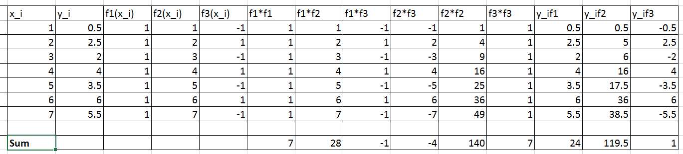
Therefore, the linear system of equations can be written as:

$\left(\begin{matrix}7&28&-1\\28&140&-4\\-1&-4&7\end{matrix}\right) \left(\begin{array}{c}a_1\\a_2\\a_3\end{array}\right)=\left(\begin{array}{c}24\\119.5\\1\end{array}\right)$

Solving the above system yields $a_1=0.16369$ , $a_2=0.83929$ , $a_3=0.64583$ . Therefore, the best-fit model has the form:

$y(x)=0.16369+0.83929x+0.64583\cos{(\pi x)}$

To find the coefficient of determination, the following Microsoft Excel table for the values of $(y_i-y(x_i))^2$ and $\left(y_i-\frac{1}{n}\sum_{i=1}^ny_i\right)^2$ is used:

linearfittable2
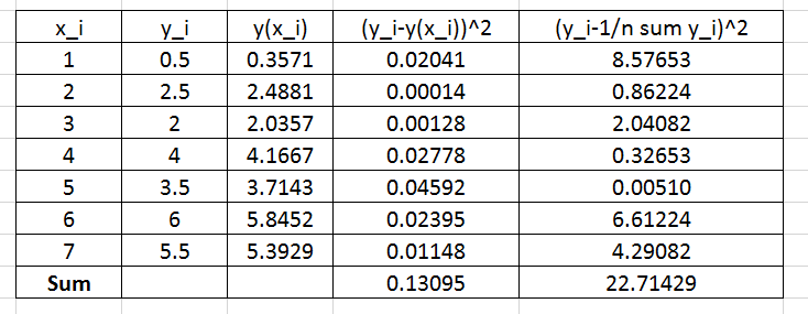
Therefore:

$R^2=1-\frac{0.13095}{22.71429}=0.994234$

$R^2$ is very close to 1 indicating a very good fit!

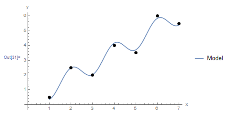
The Mathematica function LinearModelFit[Data,{functions},x] does the above computations and provides the required model. The equation of the model can be retrieved using the built-in function Normal and the $R^2$ can also be retrieved as shown in the code below. The final plot of the model vs. the data is shown below as well.

linearfit2

View Mathematica Code

Clear[a, b, x]
Data = {{1, 0.5}, {2, 2.5}, {3, 2}, {4, 4.0}, {5, 3.5}, {6, 6.0}, {7, 5.5}};
model = LinearModelFit[Data, {1, x, Cos[Pi*x]}, x]
y = Normal[model]
R2 = model["RSquared"]
Plot[y, {x, 1, 7}, Epilog -> {PointSize[Large], Point[Data]},  PlotLegends->{"Model"},AxesLabel -> {"x", "y"}, AxesOrigin -> {0, 0} ]

View Python Code

import numpy as np
import matplotlib.pyplot as plt
from scipy.optimize import curve_fit

Data = [[1, 0.5], [2, 2.5], [3, 2], [4, 4.0], [5, 3.5], [6, 6.0], [7, 5.5]]
def f(x, a, b, c): return a + b*x + c*np.cos(np.pi*x)
coeff, covariance = curve_fit(f, [point[0] for point in Data],
                                 [point[1] for point in Data])
print("coeff: ",coeff)
x_val = np.arange(0,7,0.01)
plt.title("%.5f + %.5fx + %.5fcos(pi*x)" % tuple(coeff))
plt.plot(x_val, f(x_val, coeff[0], coeff[1], coeff[2]))
plt.scatter([point[0] for point in Data], [point[1] for point in Data], c='k')
plt.xlabel("x"); plt.ylabel("y")
plt.grid(); plt.show()

# R squared
x = np.array([point[0] for point in Data])
y = np.array([point[1] for point in Data])
y_fit = f(x, coeff[0], coeff[1], coeff[2])
ss_res = np.sum((y - y_fit)**2)
ss_tot = np.sum((y - np.mean(y))**2)
r2 = 1 - (ss_res / ss_tot)
print("R Squared: ",r2)

The following links provide the MATLAB codes for implementing the generalized least squares. The function for the model in this example in provided in File 2.

MATLAB files: File 1 (ex9_2.m) File 2 (ex9_2_f.m)

Example 2

Fit a cubic polynomial to the data (1,1.93),(1.1,1.61),(1.2,2.27),(1.3,3.19),(1.4,3.19),(1.5,3.71),(1.6,4.29),(1.7,4.95),(1.8,6.07),(1.9,7.48),(2,8.72),(2.1,9.34),(2.2,11.62).

Solution

A cubic polynomial fit would have the form:

$y(x)=a_0+a_1x+a_2x^2+a_3x^3$

This is a linear combination of the functions $f_0(x)=1$ , $f_1(x)=x$ , $f_2(x)=x^2$ , and $f_3(x)=x^3$ . The following system of equations needs to be formed to solve for the coefficients $a_0$ , $a_1$ , $a_2$ , and $a_3$ :

$\begin{split}\left(\begin{matrix}\sum_{i=1}^nf_0(x_i)f_0(x_i)&\sum_{i=1}^nf_0(x_i)f_1(x_i)&\sum_{i=1}^nf_0(x_i)f_2(x_i) & \sum_{i=1}^nf_0(x_i)f_3(x_i)\\\sum_{i=1}^nf_1(x_i)f_0(x_i)&\sum_{i=1}^nf_1(x_i)f_1(x_i)&\sum_{i=1}^nf_1(x_i)f_2(x_i) & \sum_{i=1}^nf_1(x_i)f_3(x_i)\\\sum_{i=1}^nf_2(x_i)f_0(x_i)&\sum_{i=1}^nf_2(x_i)f_1(x_i)&\sum_{i=1}^nf_2(x_i)f_2(x_i) & \sum_{i=1}^nf_2(x_i)f_3(x_i)\\\sum_{i=1}^nf_3(x_i)f_0(x_i)&\sum_{i=1}^nf_3(x_i)f_1(x_i)&\sum_{i=1}^nf_3(x_i)f_2(x_i) & \sum_{i=1}^nf_3(x_i)f_3(x_i)\\\end{matrix}\right)&\left(\begin{array}{c}a_0\\a_1\\a_2\\a_3\end{array}\right)\\&=\left(\begin{array}{c}\sum_{i=1}^ny_if_0(x_i)\\\sum_{i=1}^ny_if_1(x_i)\\\sum_{i=1}^ny_if_2(x_i)\\\sum_{i=1}^ny_if_3(x_i)\end{array}\right)\end{split}$

The following Microsoft Excel tables are used to find the entries of the above linear system of equations:

example21
example22

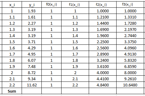
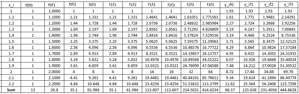
Therefore, the linear system of equations can be written as:

$\left(\begin{matrix}13&20.8&35.1&61.984\\20.8&35.1&61.984&113.607\\35.1&61.984&113.607&214.502\\61.984&113.607&214.502&414.623\end{matrix}\right)\left(\begin{array}{c}a_0\\a_1\\a_2\\a_3\end{array}\right)=\left(\begin{array}{c}68.37\\123.638\\231.4056\\444.8628\end{array}\right)$

Solving the above system yields $a_0=-1.6247$ , $a_1=6.6301$ , $a_2=-5.7273$ , and $a_3=2.46212$ . Therefore, the best-fit model has the form:

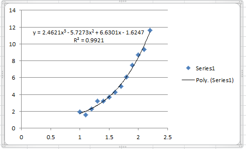
$y=-1.6247+6.6301x-5.7273x^2+2.46212x^3$

The following graph shows the Microsoft Excel plot with the generated cubic trendline. The trendline equation generated by Excel is the same as the one above.

example23

To find the coefficient of determination, the following Microsoft Excel table for the values of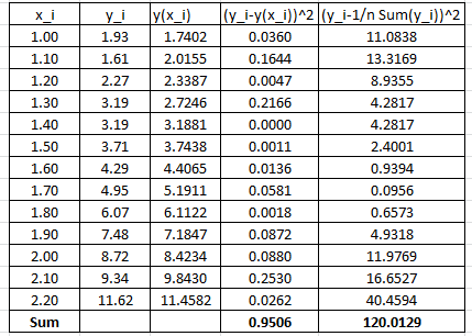 $(y_i-y(x_i))^2$ and $\left(y_i-\frac{1}{n}\sum_{i=1}^ny_i\right)^2$ is used:
example24

Therefore:

$R^2=1-\frac{0.9506}{120.0129}=0.9921$

Which is similar to the one produced by Microsoft Excel. Alternatively, the following Mathematica code does the above computations to produce the model and its $R^2$ .

View Mathematica Code

Data = {{1, 1.93}, {1.1, 1.61}, {1.2, 2.27}, {1.3, 3.19}, {1.4,3.19}, {1.5, 3.71}, {1.6, 4.29}, {1.7, 4.95}, {1.8, 6.07}, {1.9,7.48}, {2, 8.72}, {2.1, 9.34}, {2.2, 11.62}};
model = LinearModelFit[Data, {1, x, x^2, x^3}, x]
y = Normal[model]
R2 = model["RSquared"]
Plot[y, {x, 1, 2.2}, Epilog -> {PointSize[Large], Point[Data]}, PlotLegends -> {"Model"}, AxesLabel -> {"x", "y"}, AxesOrigin -> {0, 0} ]

View Python Code

import numpy as np
from scipy import stats
import matplotlib.pyplot as plt

Data = [[1, 1.93], [1.1, 1.61], [1.2, 2.27], [1.3, 3.19], [1.4,3.19], [1.5, 3.71], [1.6, 4.29], [1.7, 4.95], [1.8, 6.07], [1.9,7.48], [2, 8.72], [2.1, 9.34], [2.2, 11.62]]
coeff = np.polyfit([point[0] for point in Data],
                   [point[1] for point in Data], 3)
print("coeff: ",coeff)
slope, intercept, r_value, p_value, std_err = stats.linregress([point[0] for point in Data],
                                                               [point[1] for point in Data])
print("R Squared: ",r_value**2)
y = np.poly1d(coeff)
x = np.linspace(1, 2.2)
plt.plot(x, y(x),label="Model")
y = [str(round(i,4)) for i in list(y)]
plt.title(y[0]+"x**3 + "+y[1]+"x**2 + "+y[2]+"x + "+y[3])
plt.scatter([point[0] for point in Data],[point[1] for point in Data], c='k')
plt.xlabel("x"); plt.ylabel("y")
plt.legend(); plt.grid(); plt.show()

The following links provide the MATLAB codes for implementing the cubic polynomial fit. The function for the model in this example in provided in File2.

MATLAB files: File 1 (ex9_3.m) File 2 (ex9_3_f.m)