Engineering at Alberta Courses » Euler Bernoulli Beam

Plane Beam Approximations: Euler Bernoulli Beam

Learning Outcomes

Reproduce the derivation of the equilibrium equation of the Euler Bernoulli beam.
Describe the three basic assumptions for the equilibrium equation of the Euler Bernoulli beam.
Identify the relationship between the load, displacement, bending moment, and shear force.
Compute the bending moment, the shear force, the stress distribution, and the strain distribution in a beam by solving the differential equation of equilibrium.

There are three basic assumptions for an Euler Bernoulli beam that will be used to derive the equations. These are:

Plane sections perpendicular to the neutral axis before deformation stay plane and perpendicular to the neutral axis after deformation (Figure 1).
The deformations are small.
The beam is linear elastic isotropic and Poisson’s ratio effects are ignored.

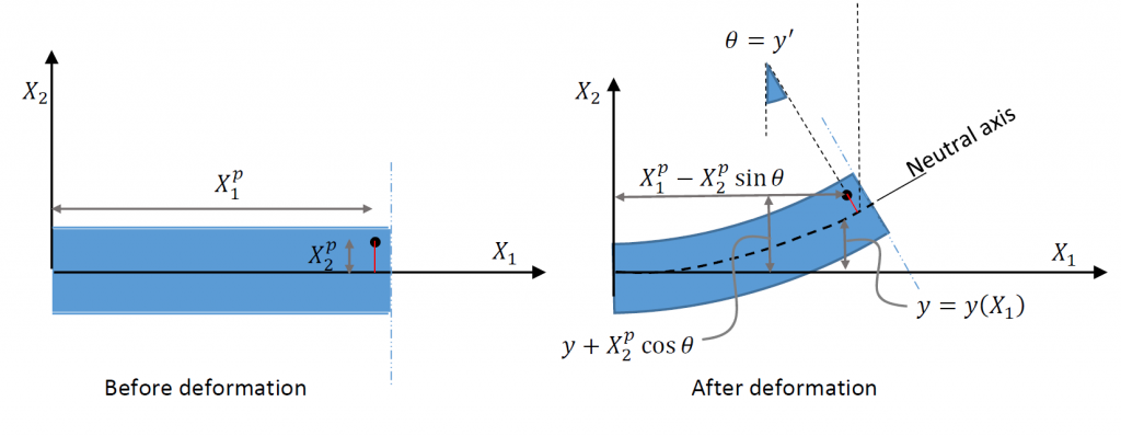
BeamDeformation-1024x398 — Figure 1. Deformation assumption for beams. The black dot represents an arbitrary point before and after deformation. Plane sections perpendicular to the neutral axis remain plane and perpendicular to the neutral axis after deformation. The coordinates of the point after deformation can be obtained accordingly.

The beam is assumed to lie such that its long axis is aligned with $X_1$ . The deformation is controlled by a function $y(X_1)$ which describes the deformation of the neutral axis (Figure 1). The first assumption allows the calculation of the small strain matrix at every point. The coordinates of an arbitrary point $p$ before deformation are given by:

$X=\left(\begin{array}{c}X_1^p\\X_2^p\\X_3^p\end{array}\right)$

Ignoring any effect due to Poisson’s ratio, the coordinates of the point $p$ after deformation (Figure 1) are given by:

$x=\left(\begin{array}{c}X_1^p-X_2^p\sin{\theta}\\y+X_2^p\cos{\theta}\\X_3^p\end{array}\right)$

The second assumption (small deformation) allows the approximations $\theta\approx \sin{\theta}\approx \tan{\theta} and \cos{\theta}\approx 1$ . Therefore, the displacement function after incorporating the small deformations assumption is given by:

$u=x-X=\left(\begin{array}{c}-X_2^p\theta\\y\\0\end{array}\right)$

We can drop the superscript $p$ since this applies to any arbitrary point. We also note that $y'=\tan{\theta}\approx \theta$ . Therefore, the displacement function has the form:

$u=x-X=\left(\begin{array}{c}-X_2\frac{\mathrm{d}y}{\mathrm{d}X_1}\\y\\0\end{array}\right)$

We remind the reader that $y$ is a function of $X_1$ only and so is its derivative. Therefore, The gradient of the displacement matrix is given by:

$\nabla u=\left(\begin{matrix}-X_2\frac{\mathrm{d}^2y}{\mathrm{d}X_1^2} & -\frac{\mathrm{d}y}{\mathrm{d}X_1} & 0 \\\frac{\mathrm{d}y}{\mathrm{d}X_1} & 0 & 0\\0&0&0\end{matrix}\right)$

Therefore, the small strain matrix has the form:

$\varepsilon=\frac{1}{2}\left(\nabla u + \nabla u^T\right)=\left(\begin{matrix}-X_2\frac{\mathrm{d}^2y}{\mathrm{d}X_1^2} & 0 & 0 \\0 & 0 & 0\\0&0&0\end{matrix}\right)$

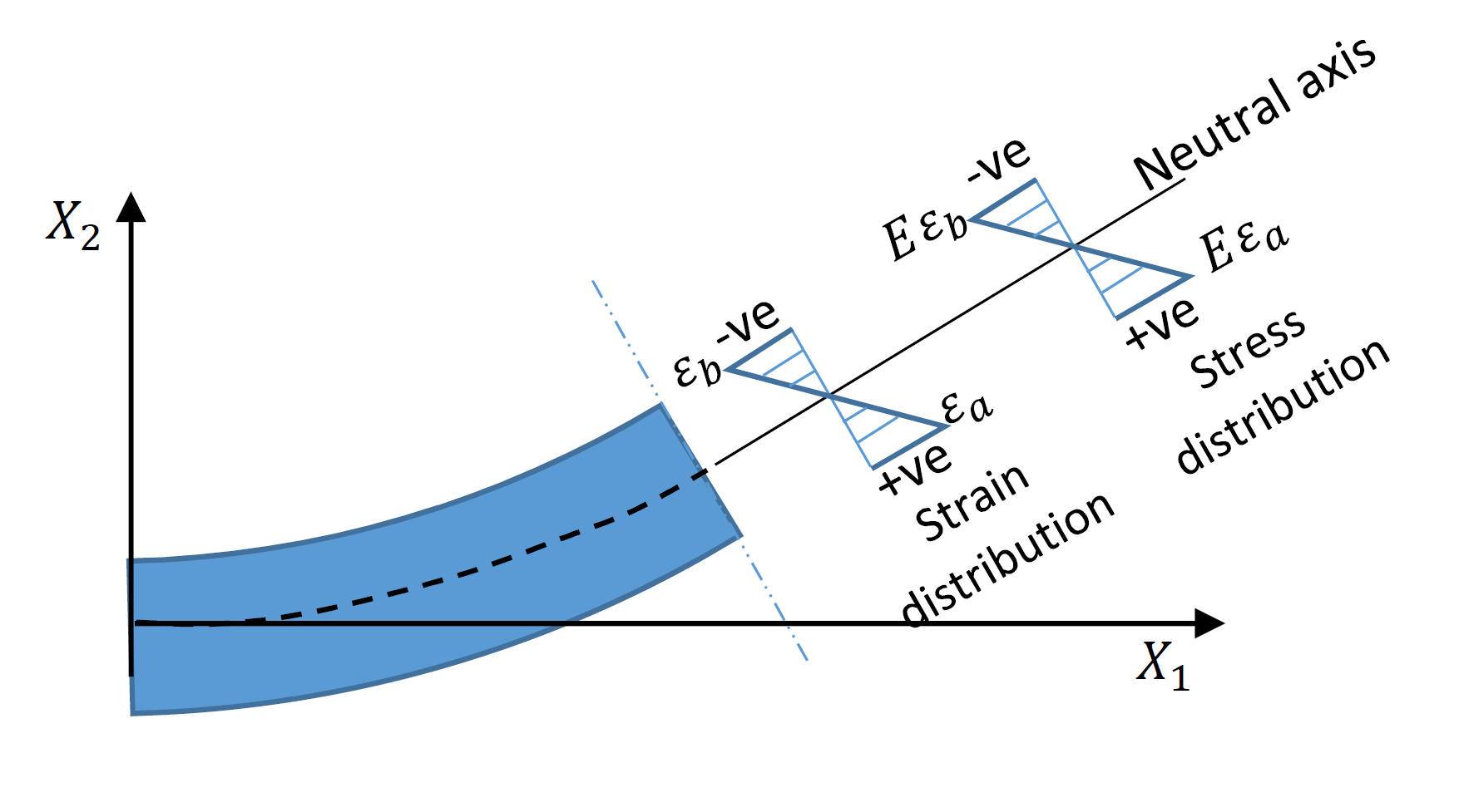
In essence, the deformation assumptions result in all of the strain components being zero except for $\varepsilon_{11}$ . Furthermore, we will look carefully at the variation of $\varepsilon_{11}$ on a given cross section. For a given cross section of the beam we have X_1 is equal to constant. Therefore, the quantity $\frac{\mathrm{d}^2y}{\mathrm{d}X_1^2}$ is constant on the cross section and therefore $\varepsilon_{11}$ is linear in the vertical direction (Figure 2). The value of $\varepsilon_{11}$ is equal to zero at the neutral axis $X_2=0$ . The positive convention for $y$ and for $y'$ lead to a positive strain below the neutral axis with the maximum positive value $\varepsilon_a$ at the bottom fibre of the cross section. The positive convention also leads to a negative strain above the neutral axis with the maximum negative value $\varepsilon_b$ at the top fibre of the cross section. Using the linear elastic constitutive relationship for the beam material and ignoring Poisson’s ratio lead to the same distribution for $\sigma_{11}=E\varepsilon_{11}$ (Figure 2). Therefore, the normal stress component distribution on the cross section is given by:

(1) $\begin{equation*}\sigma_{11}=-EX_2\frac{\mathrm{d}^2y}{\mathrm{d}X_1^2}\end{equation*}$

BeamDistribution — Figure 2. The linear distribution of the longitudinal strain component $\varepsilon_{11}$ and the longitudinal stress component $\sigma_{11}$ on the beam cross section.

Internal Forces

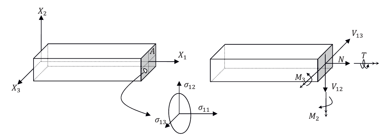
The deformation assumption in beams allows considering only the deformation of the neutral axis. In particular, the deformation of the beam is controlled by the unknown function $y(X_1)$ which is the vertical deformation of the neutral axis. We can also look at the forces acting on the cross section that is perpendicular to the neutral axis. These forces are termed: “Internal Forces” and can be obtained by integrating the various stress components acting on the cross section under consideration (Figure 3). For a beam in plane, only two internal forces are considered, the bending moment $M_3(X_1)=M(X_1)$ , and the shearing force $V_{12}(X_1)=V(X_1)$ . The positive convention for these internal forces is shown in Figure 3. $M(X_1)$ can be obtained by integrating the stress component $\sigma_{11}$ on the cross section:

$M=\int \int \! -X_2\sigma_{11} \,\mathrm{d}X_2\mathrm{d}X_3$

The negative sign is introduced to keep the positive convention for $M$ causing compression on the top fibre of the beam. By substituting for $\sigma_{11}$ using Equation 1, the moment can be calculated as:

(2) $\begin{equation*} M=\int \int \! EX_2^2\frac{\mathrm{d}^2y}{\mathrm{d}X_1^2} \,\mathrm{d}X_2\mathrm{d}X_3=EI\frac{\mathrm{d}^2y}{\mathrm{d}X_1^2} \end{equation*}$

where I is the moment of inertia of the beam calculated according to the formula:

$I=\int \int \! X_2^2 \,\mathrm{d}X_2\mathrm{d}X_3$

Equation 1 and Equation 2 can be used to find the relationship between the internal bending moment $M$ and the stress component $\sigma_{11}$ on the cross section:

(3) $\begin{equation*} \sigma_{11}=-\frac{MX_2}{I} \end{equation*}$

Beam1 — Figure 3. Integration of stress components on the beam’s cross section to obtain the internal forces

Equilibrium Equations

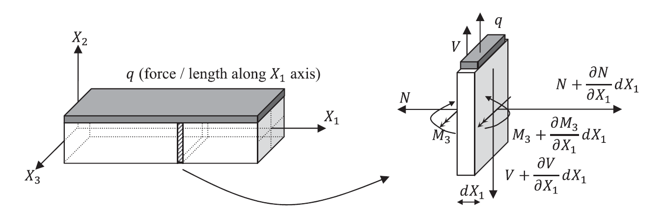
It is possible to derive the equilibrium equations for the Euler Bernoulli beam by integrating the general equilibrium equations of a continuum. However, we will follow the classical method as described in many structural analysis books following the sign convention shown in Figure 3. First, two planes that are very close to each other (separated by a small distance $\Delta X_1$ and perpendicular to the $axis X_1$ are considered. Then, by assuming that $V$ and $M$ are smooth functions of $X_1$ , then the first approximation in a Taylor’s series can be utilized to describe the changes in the internal forces between those two planes (Figure 4). The loading on the beam is assumed to be transverse in the direction of $X_2$ upwards and given by $q$ with units of load per beam length. Assuming the sum of forces in the vertical direction (direction of $X_2$ ) is equal to zero yields:

$\frac{\partial V}{\partial X_1}=q$

Similarly, assuming the sum of moments around $X_3$ is equal to zero yields:

$\frac{\partial M}{\partial X_1}=V$

Since $V$ , $q$ and $M$ are only functions of $X_1$ , the partial derivatives can be replaced with total derivatives and the equilibrium equations become:

(4) $\begin{equation*} \begin{split}\frac{\mathrm{d} V}{\mathrm{d} X_1}& =q\\ \frac{\mathrm{d} M}{\mathrm{d} X_1}& =V\end{split} \end{equation*}$

We can substitute for $M$ using Equation 2 so the equilibrium equation in terms of the displacement function $y$ and the loading $q$ becomes:

(5) $\begin{equation*} EI\frac{\mathrm{d}^4 y}{\mathrm{d} X_1^4} =q \end{equation*}$

The solution for $y$ has the following form:

$EIy=\int\int\int\int \!q \,\mathrm{d}X_1 \mathrm{d}X_1 \mathrm{d}X_1 \mathrm{d}X_1 + C_1\frac{X_1^3}{6}+C_2\frac{X_1^2}{2}+C_3X_1+C_4$

Four boundary conditions are needed to fully solve for $y$ and its derivatives. These boundary conditions can be given in terms of the displacement $y$ , the rotation $\theta=\frac{\mathrm{d}y}{\mathrm{d}X_1}$ , the bending moment $M=EI\frac{\mathrm{d}^2y}{\mathrm{d}X_1^2}$ or the shearing force $V=EI\frac{\mathrm{d}^3y}{\mathrm{d}X_1^3}$ . Note that if $q=0$ the beam can have a polynomial shape up to the third degree. For this reason, this formulation is sometimes termed: The cubic formulation.

Beam2 — Figure 4. Equilibrium Equations for the Euler Bernoulli and the Timoshenko beams subjected to transverse loading.

Shear Stress in Euler Bernoulli Beam:

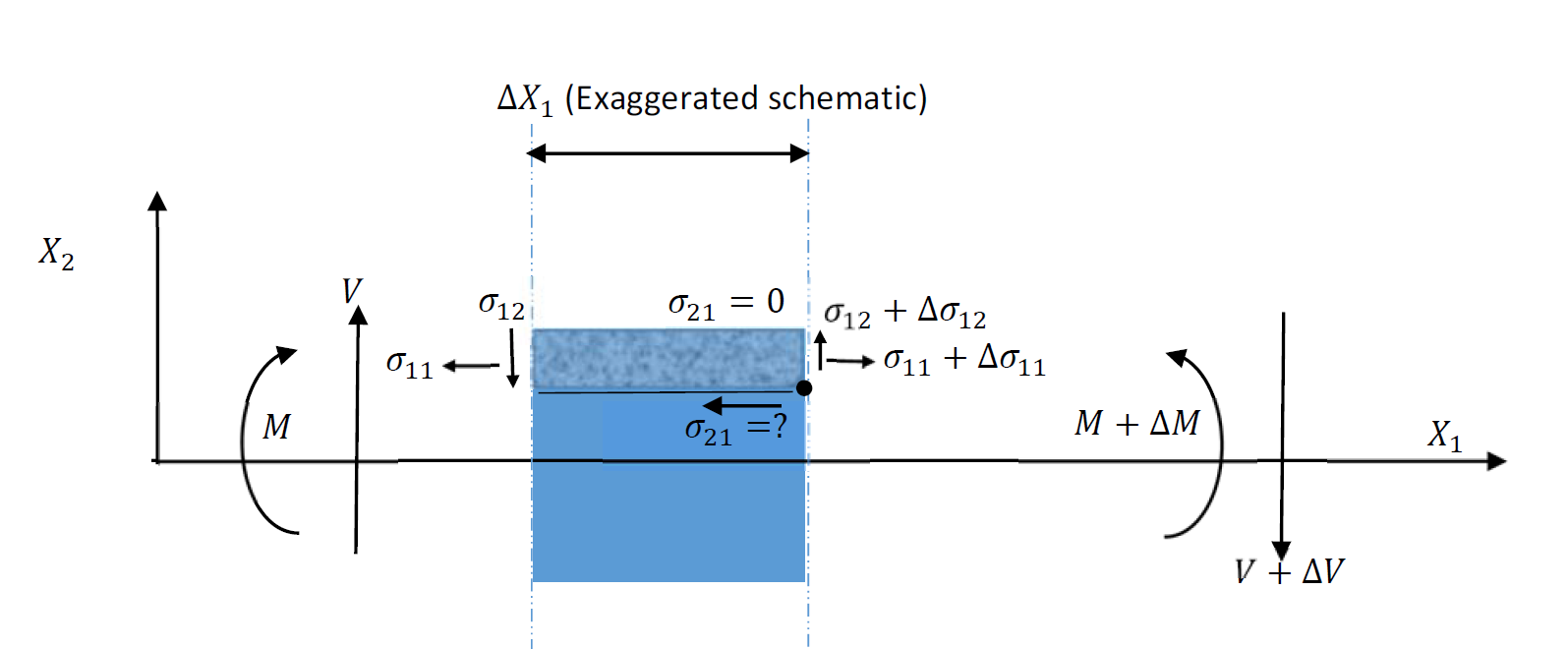
The small strain matrix obtained above for the Euler Bernoulli beam shows that the shear strains are equal to zero. However, this is an approximation that simplifies the beam model. While shear strains are directly proportional to shear stresses in linear elastic materials, for the Euler Bernoulli beam, shear stresses arise from the existence of the shearing force $V$ even though the shear strains are equal to zero. The shearing stresses associated with $V$ can be calculated by first assuming that the shear stress $\sigma_{12}$ is constant across the beam width (along the $X_3$ direction). Then, by considering a small slice in the beam with width of $\Delta X_1$ the shear stress at the point represented by the black circle in Figure 5 can be calculated by considering the equilibrium of the shaded section shown in the figure. There are three horizontal forces acting on the shaded section. On the left we have $F_1$ caused by integrating $\sigma_{11}+\Delta\sigma_{11}$ on the left cross section of the shaded area. On the right we have $F_2$ caused by integrating $\sigma_{11}$ on the right cross section of the shaded area. At the bottom we have $F_3$ caused by integrating $\sigma_{21}$ on the bottom of the shaded area. Using Equation 3 that relates $\sigma_{11}$ with $M$ , the three forces can be calculated as follows:

$\begin{split} F_1 & =\int\int\! \left(\sigma_{11}+\Delta \sigma_{11}\right)\,\mathrm{d}X_2\mathrm{d}X_3=\int\int\! -\frac{M+\Delta M}{I}X_2\,\mathrm{d}X_2\mathrm{d}X_3\\F_2 & =\int\int\! \sigma_{11} \,\mathrm{d}X_2\mathrm{d}X_3=\int\int\! -\frac{M}{I}X_2\,\mathrm{d}X_2\mathrm{d}X_3\\F_3 & = \sigma_{21}\Delta X_1 b\end{split}$

where $b$ is the width of the cross section (the width in the direction of $X_3$ ). Equilibrium dictates:

$F_1-F_2-F_3=0$

Therefore,

$F_1-F_2-F_3=\int\int\! -\frac{\Delta M}{I}X_2\,\mathrm{d}X_2\mathrm{d}X_3-\sigma_{21}\Delta X_1 b=0$

We will use the equality: $\Delta M\approx\frac{\mathrm{d}M}{\mathrm{d}X_1}\Delta X_1=V\Delta X_1$ . Therefore:

$\int\int\! -\frac{V}{I}\Delta X_1 X_2\,\mathrm{d}X_2\mathrm{d}X_3-\sigma_{21}\Delta X_1 b=0$

Since $V$ , $I$ , and $\Delta X_1$ are not functions of $X_2$ or $X_3$ , they can be brought outside the integral. Denote $Q$ to be the moment of the area defined by:

$Q=\int\int\! X_2\,\mathrm{d}X_2\mathrm{d}X_3$

Therefore:

$\sigma_{21}=-\frac{VQ}{Ib}$

Since $\sigma_{21}$ is equal to $\sigma_{12}$ , the shear stress on the cross section at the point in question is equal to:

(6) $\begin{equation*}\sigma_{12}=-\frac{VQ}{Ib}\end{equation*}$

A similar proof can be found in the Mechanics ebook here.

Discrepancies of The Beam Theory:

The Euler Bernoulli beam model is a simple approximation. While it is very successful because of it simplicity and practicality, it has a few discrepancies. One discrepancy is that the shear stress is not associated with any shear strains. The second discrepancy is that the calculated stresses, while they satisfy equilibrium in a holistic sense, they don’t necessarily satisfy the equilibrium equation of the continuum at a local sense. In particular, the equation of horizontal equilibrium of the continuum is:

$\frac{\partial \sigma_{11}}{\partial X_1}+\frac{\partial \sigma_{21}}{\partial X_2}+\frac{\partial \sigma_{31}}{\partial X_3}=0$

Notice that $\sigma_{31}$ is assumed to be zero and that we are using the undeformed coordinates $X_i$ since small deformations are assumed. Also, no body forces are assumed to be acting on the beam. By setting $\sigma_{31}=0$ and substituting for $\sigma_{11}$ and $\sigma_{21}$ using Equation 3 and Equation 6 respectively, we get the following:

$\frac{\partial \sigma_{11}}{\partial X_1}+\frac{\partial \sigma_{21}}{\partial X_2}=\frac{\partial \left(-\frac{MX_2}{I}\right)}{\partial X_1}-\frac{\partial \frac{VQ}{Ib}}{\partial X_2}$

Assuming $I$ is constant along $X_1$ and since $V$ and $I$ are functions only of $X_1$ we get:

$\frac{\partial \sigma_{11}}{\partial X_1}+\frac{\partial \sigma_{21}}{\partial X_2}=-\frac{X_2}{I}\frac{\partial M}{\partial X_1}-\frac{V}{I}\frac{\partial \frac{Q}{b}}{\partial X_2}$

Therefore:

$\frac{\partial \sigma_{11}}{\partial X_1}+\frac{\partial \sigma_{21}}{\partial X_2}=\frac{V}{I}\left(-X_2 -\frac{\partial \frac{Q}{b}}{\partial X_2}\right)$

The left hand side is only equal zero if $b$ is constant (i.e., rectangular cross section). Otherwise, the left hand side calculation for any cross section other than a rectangle will give nonzero values, i.e., equilibrium is not necessarily satisfied!

Video

Quiz 25 – Euler-Bernoulli Beam

Solution Guide

Page Comments

Aliu Abdul-Hamid says:

August 10, 2021 at 8:51 pm

Thank you very much for this educative video. I would be happy for clarification on how you obtained the vertical position of the deformed point as y + X2pcos(theta). From my understanding, since plane sections remain plane after deformation, X2p will remain perpendicular to the neutral axis and I find that not to be the hypotaneous if a right angle triangle is drawn. The vertical line drawn to connect point X2p to the neutral axis seems to me to be the hypotaneus. From my calculation, the vertical displacement will be X2p/cos(theta). I do however understand how the horizontal distance changes. My understanding is that, a different right-angle triangle is used for the horizontal displacement. The triangle used was obtained by connecting a horizontal line between the point of intersection of the line connecting X2p to the neutral axis and the vertical line drawn from point X2p. I would be grateful if you could connect to explain your derivation better to me. Thank you

Reply
1. Samer Adeeb says:
  
  August 11, 2021 at 9:26 am
  
  After deformation, the line drawn from the point to the neutral axis is no longer vertical as inferred from figure 2 above. The distance between the point and the neutral axis along that inclined line is equal to X2p. This inclined distance is resolved into two components: horizontal and vertical. The vertical distance becomes X2p*Cos(theta).
  
  Reply
  1. Aliu Abdul-Hamid says:
    
    August 12, 2021 at 9:20 am
    
    Thank you Prof. for the response. I have sent you an email with an attachment. Kindly review.
Yaman Boluk says:

December 30, 2023 at 2:54 pm

Excellent learning material. I would like to know which Bernoulli brother had it. Older Jacob or younger Johann one. There was a big rivalry among them.

Reply
1. Samer Adeeb says:
  
  December 30, 2023 at 2:55 pm
  
  Sorry, Dr. Boluk. I don’t know the answer to this.
  
  Reply
2. Yaman Boluk says:
  
  December 30, 2023 at 3:01 pm
  
  I guess he was Johann’s second son Daniel.
  
  Reply
Yaman Boluk says:

December 30, 2023 at 3:00 pm

I guess Johann’s second son Daniel was the Bernoulli in the equation’s name. He worked on mechanics of flexible elastic bodies with Euler.

Reply