
Linear Maps Between Vector Spaces: Basic Definitions
Learning Outcomes
- Describe matrices as linear functions from one space to another. Describe the matrix as a representation of this function in a particular ONB.
- Calculate the Kernel of simple matrices. Describe what the Kernel represents. Define an invertible matrix as one that has one element in the kernel.
- Calculate the components of a matrix in various ONBs
- Compute matrix multiplication
- Differentiate between an invertible (bijective) matrix and one that is a non-invertible matrix using the geometry of a linear map.
- Calculate the determinant of a 2×2 and a 3×3 matrix. Explain that the determinant is a measure of whether a matrix is invertible or not.
- Identify and apply the properties of the determinant function.
- Define eigenvalues and eigenvectors. Identify the properties of the eigenvalues and eigenvectors.
- Eigenvalues and Eigenvectors: Visualize the geometry of eigenvalues and eigenvectors (The online tool helps the visualization of the eigenvector as the vector that does not change direction when transformed by the matrix).
Compute eigenvalues and eigenvectors.
Linear Maps
A linear map  between two vectors spaces
  and
and  is a function
  such that
  :
:
![\[ T(\alpha u + \beta v)=\alpha T(u)+\beta T(v) \]](https://engcourses-uofa.ca/wp-content/ql-cache/quicklatex.com-ae7c9c01d31a3012b87dc8243164be4a_l3.png "Rendered by QuickLaTeX.com")
Notice that the addition of two linear maps and their multiplication by scalars produce a linear map as well, which imply that the set of linear maps is also a linear vector space.
It is important not to confuse linear maps with affine maps. For example, the function  defined such that
  is not a linear map but rather an affine map.
  is not a linear map since in general
  . On the other hand, the function
  defined such that
  is indeed a linear map.
Tensors
Linear maps between finite dimensional linear vector spaces is one example of functions that are referred to as Tensors. Tensor analysis provides a natural and concise mathematical tool for the analysis of various engineering problems, in particular, solid mechanics. For a detailed description of tensors, refer to the Wolfram article on tensors.
According to wikipedia, the origin of the word “Tensors” dates back to the nineteenth century when it was introduced by Woldemar Voigt. It is likely that the word originated because one of the early linear operators introduced was the symmetric Cauchy stress matrix which functions to convert area vectors to force vectors. At the time, perhaps the scientists were interested in things that “stretch” and thus, the word “Tensor” from the Latin route “Tendere” came about.
Kernel of Linear Maps
Let T be a linear map between two vector spaces and . Then, the kernel of or  is the set of all vectors that are mapped into the zero vector, i.e.:
![\[ \ker(T)=\{x\in V|T(x)=0\} \]](https://engcourses-uofa.ca/wp-content/ql-cache/quicklatex.com-35fd4108a5a5446bad3ac6ae18b3b58c_l3.png "Rendered by QuickLaTeX.com")
For example, consider the linear map  defined such that
  ,
,  . Then, the kernel of this linear map consists of al the vectors in
  that are mapped to zero, i.e., the vectors whose components
  and
and  satisfy:
![\[ 5x_1 + 6x_2=0\Rightarrow x_1=-1.2x_2 \]](https://engcourses-uofa.ca/wp-content/ql-cache/quicklatex.com-b7e70b12c5336e646ce90cfe8fab02cb_l3.png "Rendered by QuickLaTeX.com")
There are infinitely many vectors that satisfy this condition. The set of all those vectors is given as:

Matrix Representation of Linear Maps
The matrix representation of linear maps is the most convenient way to represent linear maps when orthonormal basis sets are chosen for the underlying vector spaces. Consider the linear map  . Let
. Let  and
and  be the orthonormal basis sets for
  and
and  respectively. Then, because of the linearity of the map, the map is indeed well defined by the components of the vectors
  . Since
  we can assume that it has
  components which can be denoted as follows:
![\[ Te_j=T_{1j} e'_1+T_{2j} e'_2+\cdots+T_{mj} e'_m=\sum_{i=1}^m T_{ij}e'_i \]](https://engcourses-uofa.ca/wp-content/ql-cache/quicklatex.com-d43afedaca0078300a8eabb68c39ad30_l3.png "Rendered by QuickLaTeX.com")
 and its image under T has the form:
![\[ T\sum_{j=1}^n(x_je_j)=\sum_{j=1}^n(x_jTe_j)=\sum_{i=1}^m \sum_{j=1}^n T_{ij}x_j e'_i \]](https://engcourses-uofa.ca/wp-content/ql-cache/quicklatex.com-25ab8f3ad814d44d7f37601d212f7efd_l3.png "Rendered by QuickLaTeX.com")
![\[ Tx= \left( \begin{array}{cccc} T_{11}&T_{12}&\cdots&T_{1n}\\ T_{21}&T_{22}&\cdots&T_{2n}\\ \vdots & \vdots &\ddots &\vdots\\ T_{m1}&T_{m2}&\cdots &T_{mn} \end{array} \right) \left( \begin{array}{cc} x_1\\ x_2\\ \vdots\\ \vdots\\ x_n \end{array} \right) \]](https://engcourses-uofa.ca/wp-content/ql-cache/quicklatex.com-7120c2a55ed8a9643dc31fab730debca_l3.png "Rendered by QuickLaTeX.com")
are the column vectors of the matrix representation .
Matrix Representation and Change of Basis
The components of the matrix representation of defined above depend on the choice of the orthonormal basis sets for each vector space. For the discussion in this section, we will restrict ourselves to square matrices, i.e., linear maps between vector spaces of the same dimension.
Let  . Let be the chosen orthonormal basis set for both vector spaces and let
  be another orthonormal basis set and let
  be the matrix of coordinate transformation as defined in the Change of Basis section. The matrix representation of when
  is chosen as the basis set is denoted by
  . The relationship between and can be obtained as follows:
Let  , denote
  . Let
. Let  and
and  denote the representation of
  and
and  when is chosen as the coordinate system. Therefore in each coordinate system we have:
![\[ y'=T'x'\hspace{10mm} y=Tx \]](https://engcourses-uofa.ca/wp-content/ql-cache/quicklatex.com-eeda7d186f289c896fd7585b6da68250_l3.png "Rendered by QuickLaTeX.com")
![\[ x'=Qx\hspace{10mm}y'=Qy \]](https://engcourses-uofa.ca/wp-content/ql-cache/quicklatex.com-d815e011d3feeb4240be2c68e0363368_l3.png "Rendered by QuickLaTeX.com")
![\[ y'=T'x'=T'Qx\hspace{10mm}\text{ and }\hspace{10mm}y'=Qy=QTx\Rightarrow T'Qx=QTx \]](https://engcourses-uofa.ca/wp-content/ql-cache/quicklatex.com-704200528ca5da19abcf07dd2889a809_l3.png "Rendered by QuickLaTeX.com")
This is true for every , therefore:
![\[ T'Q=QT\Rightarrow T'=QTQ^T \]](https://engcourses-uofa.ca/wp-content/ql-cache/quicklatex.com-03e11b1ba2a380e157fa13bb52ddd626_l3.png "Rendered by QuickLaTeX.com")
In the following tool, you can choose the components of the matrix  and the vector
  along with an angle
  of the counterclockwise rotation of the coordinate system. The tool then applies the transformation of coordinates from the coordinate system
  , to
, to  where
where  are vectors rotated by counterclockwise from
  , and
, and  . On the left hand side, the tool draws the vector
  in blue, the vector
  in red, the original coordinate system in black, and the vectors of the new coordinate system in dashed black. At the bottom of the left hand side drawing you will find the expressions for
  and
and  using the basis set
  . On the right hand side, the tool draws the vectors
  in blue,
  in red, and the new coordinate system in black. At the bottom of the right hand side, you will find the expressions for
  and
and  using the basis set . You can also check out the external tool built in MecsimCalc for changes of basis.
Similarly, the following tool is for three dimensional Euclidean vector spaces. The new coordinate system  is obtained by simultaneously applying a counterclockwise rotation
  , and
, and  around the first, second, and third coordinate system axis, respectively. The view can be zoomed, rotated or panned by the mouse scroll wheel, holding down the left mouse button and moving the mouse, and holding down the right mouse button and moving the mouse.
Tensor Product
Let  and
and  . The tensor product denoted by
  is a linear map
  defined such that
  :
:
![\[ (v\otimes u) x=(x\cdot u)v \]](https://engcourses-uofa.ca/wp-content/ql-cache/quicklatex.com-cf51e7306b33e08258439924baa1a7ee_l3.png "Rendered by QuickLaTeX.com")
In simple words, the tensor product defined above utilizes the linear dot product operation and a fixed vector  to produce a real number using the expression
  , which is conveniently a linear function of . The resulting number is then multiplied by the vector .
Obviously, the tensor product of vectors belonging to vector spaces of dimensions higher than 1 are not invertible, in fact, the range of is one dimensional (why?)!
The following are some of the properties of the tensor product that can be deduced directly from the definition and the properties of the dot product operation,  :
:
![\[ (\alpha u + \beta v)\otimes w=\alpha (u\otimes w) + \beta (v\otimes w) \]](https://engcourses-uofa.ca/wp-content/ql-cache/quicklatex.com-0f7b22569cf3286596fa46bb8deb3aa9_l3.png "Rendered by QuickLaTeX.com")
![\[ w\otimes(\alpha u + \beta v)=\alpha (w\otimes u) + \beta (w\otimes v) \]](https://engcourses-uofa.ca/wp-content/ql-cache/quicklatex.com-d61cd46a9bcb3f45029361d33cc67e63_l3.png "Rendered by QuickLaTeX.com")
![\[ (a\otimes u)(v\otimes w)=(u\cdot v)(a\otimes w) \]](https://engcourses-uofa.ca/wp-content/ql-cache/quicklatex.com-4156a3ff306a18623193ed86e5b9af9a_l3.png "Rendered by QuickLaTeX.com")
![\[ T\left(u\otimes w\right)=Tu\otimes w \]](https://engcourses-uofa.ca/wp-content/ql-cache/quicklatex.com-36c1dc4d50f5b5d96f1c172712f58563_l3.png "Rendered by QuickLaTeX.com")
 , and
, and  are three orthonormal vectors, then:
![\[ I=p\otimes p + q\otimes q + r\otimes r \]](https://engcourses-uofa.ca/wp-content/ql-cache/quicklatex.com-a7174a2ab816edd274fe89bb17d127ff_l3.png "Rendered by QuickLaTeX.com")
Matrix Representation of the Tensor Product
Let  and consider the tensor product . Consider the orthonormal basis set
  . Then, the tensor product can be expressed in component form as follows:
![\[ v\otimes u=(v_1e_1+v_2e_2+v_3e_3)\otimes (u_1e_1+u_2e_2+u_3e_3)=\sum_{i,j=1}^3 v_iu_j (e_i\otimes e_j) \]](https://engcourses-uofa.ca/wp-content/ql-cache/quicklatex.com-21ed9ae8ec3be3788ef9e537ceab5a03_l3.png "Rendered by QuickLaTeX.com")
Now,  we have:
![\[ (v\otimes u)x=\sum_{i,j,k=1}^3 v_iu_j (e_i\otimes e_j)(x_ke_k)=\sum_{i,j=1}^3 v_iu_j x_j e_i \]](https://engcourses-uofa.ca/wp-content/ql-cache/quicklatex.com-c59db8a9f1e0cd12fab531ac201c2ace_l3.png "Rendered by QuickLaTeX.com")
Which, can be represented in matrix form as follows:
![\[ (v\otimes u)x= \left( \begin{array}{cc} \sum_{j=1}^3 v_1u_j x_j\\ \sum_{j=1}^3 v_2u_j x_j\\ \sum_{j=1}^3 v_3u_j x_j \end{array} \right)= \left( \begin{array}{ccc} v_1u_1&v_1u_2&v_1u_3\\ v_2u_1&v_2u_2&v_2u_3\\ v_3u_1&v_3u_2&v_3u_3 \end{array} \right) \left( \begin{array}{cc} x_1\\ x_2\\ x_3 \end{array} \right) \]](https://engcourses-uofa.ca/wp-content/ql-cache/quicklatex.com-a474fcd7f93606af4345151256c6e7bc_l3.png "Rendered by QuickLaTeX.com")
Tensor Product Representation of Linear Maps
A linear map can be decomposed into the sum of multiple tensor products. For example, one can think of a linear map between three dimensional vector spaces, as the sum of three tensor products:
![\[ T=u\otimes x +v\otimes y + w\otimes z \]](https://engcourses-uofa.ca/wp-content/ql-cache/quicklatex.com-246f900ca991591433ea45ab5aa2221a_l3.png "Rendered by QuickLaTeX.com")
 and
and  has to be linearly independent (why?).
There is a direct relationship between the tensor product representation and the matrix representation as follows: let  and let be an orthonormal basis set for both vector spaces, then, :
![\[ Tx=T\sum_{j=1}^3(x_je_j)=\sum_{j=1}^3(x_jTe_j)=\sum_{i=1}^3 \sum_{j=1}^3 T_{ij}x_j e_i=\sum_{i=1}^3 \sum_{j=1}^3 T_{ij}(x\cdot e_j) e_i=\sum_{i=1}^3 \sum_{j=1}^3 T_{ij}(e_i\otimes e_j) x \]](https://engcourses-uofa.ca/wp-content/ql-cache/quicklatex.com-44ea5b97dec7a3ea4e34fbf55217851e_l3.png "Rendered by QuickLaTeX.com")
can be represented as the sum of nine tensor product components
![\[ T=\sum_{i=1}^3 \sum_{j=1}^3 T_{ij}(e_i\otimes e_j) \]](https://engcourses-uofa.ca/wp-content/ql-cache/quicklatex.com-cdd73a275a994e8b97eec21eb5e247be_l3.png "Rendered by QuickLaTeX.com")
Video
See “Tensor Product” Video here
The Set of Linear Maps
In these pages, the notation  is used to denote the set of linear maps between and . i.e.,:
![\[ \mathbb{B}(\mathbb{R}^n,\mathbb{R}^m)=\{T:\mathbb{R}^n\rightarrow \mathbb{R}^m|T \text{ is linear}\} \]](https://engcourses-uofa.ca/wp-content/ql-cache/quicklatex.com-2e489e8904a526b5585c8a274c755312_l3.png "Rendered by QuickLaTeX.com")
 is used to denote the set of linear maps between and . i.e.,
![\[ \mathbb{B}(\mathbb{R}^n)=\{T:\mathbb{R}^n\rightarrow \mathbb{R}^n|T \text{ is linear}\} \]](https://engcourses-uofa.ca/wp-content/ql-cache/quicklatex.com-516e7cec42605f0e6647117ff36e0cc3_l3.png "Rendered by QuickLaTeX.com")
 matrices denoted
  to denote
The Algebraic Structure of The Set of Linear Maps
In addition to being a vector space, the elements of the sets of linear maps has an algebraic structure arising naturally from the composition operation. Let  and
and  , then, the composition map
  is also a linear map since
 ,
, :
:
![\[ \begin{split} T(\alpha x + \beta y)&=V\circ U(\alpha x + \beta y)\\ &=V(U((\alpha x + \beta y)))\\ &=V(\alpha U(x)+\beta U(y))\\ &=\alpha V(U(x)) + \beta V(U(y))\\ &=\alpha T(x) + \beta T(y) \end{split} \]](https://engcourses-uofa.ca/wp-content/ql-cache/quicklatex.com-fa6e30c19d4f56094f12dae56fe567e8_l3.png "Rendered by QuickLaTeX.com")
. If  and
and  are the matrices associated with the linear maps
  and respectively, then, the components of the matrix
  associated with the linear map can be obtained from the equality:
  :
:
![\[ \begin{split} Lx&=\left( \begin{array}{c} \sum_{j=1}^nL_{1j}x_j\\ \sum_{j=1}^nL_{2j}x_j\\ \cdots\\ \sum_{j=1}^nL_{lj}x_j \end{array} \right)\\ NMx&=N\left( \begin{array}{c} \sum_{j=1}^nM_{1j}x_j\\ \sum_{j=1}^nM_{2j}x_j\\ \cdots\\ \sum_{j=1}^nM_{mj}x_j \end{array}\right) = \left( \begin{array}{c} \sum_{k=1}^m\sum_{j=1}^nN_{1k}M_{kj}x_j\\ \sum_{k=1}^m\sum_{j=1}^nN_{1k}M_{kj}x_j\\ \cdots\\ \sum_{k=1}^m\sum_{j=1}^nN_{lk}M_{kj}x_j \end{array} \right) \end{split} \]](https://engcourses-uofa.ca/wp-content/ql-cache/quicklatex.com-c97ddeeee5d2af5d5040c826de3c4ff4_l3.png "Rendered by QuickLaTeX.com")
 can be calculated from the components of and as follows:
![\[ L_{ij}=\sum_{k=1}^mN_{ik}M_{kj} \]](https://engcourses-uofa.ca/wp-content/ql-cache/quicklatex.com-0fa121e7a4e7cdc3149c61197f4f6a0e_l3.png "Rendered by QuickLaTeX.com")
 row and the
  column of is equal to the multiplication of the components in the row of by the components in the column of . Notice that the operation
  is well defined while the operation
  isn’t because of the difference in the dimensions
  of the above spaces.
However, if  , and their respective associated matrices are
  then both composition maps are well defined. The first one is the composition map
  with its associated matrix while the second is the composition map
  and its associated matrix . In general, these two maps are not identical.
The identity map  and its associated identity matrix
  is the identity element in the algebraic structure of
Bijective(Invertible) Linear Maps
In this section, we are concerned with the linear maps represented by square matrices  and whether these linear maps (linear functions) are invertible or not. Recall from the Mathematical Preliminaries section that a function
  is invertible if
  such that
  .
.  is denoted by
  . Let’s now consider the linear map (represented by a matrix ) , what are the conditions that guarantee the existence of such that
  where is the identity matrix? We will answer this question using a few statements:
Statement 1: Let be a linear map. Then  .
This statement is simple to prove. First note that since is a linear map, then
.
This statement is simple to prove. First note that since is a linear map, then  .
First, assume is injective. Since and since is injective therefore, 0 is the unique image of 0. Therefore,
.
First, assume is injective. Since and since is injective therefore, 0 is the unique image of 0. Therefore,  . For the opposite statement, assume that . We will argue by contradiction, i.e., assuming that is not injective. Therefore,
  with
with  but
but  . Since is linear we have
  . Therefore,
  which is a contradiction. Therefore is injective.
◼
Statement 2: Let be a linear map. Then  .
First assume that is invertible, therefore, is injective. Statement 1 asserts then that .
Assume now that . Therefore, from statement 1, is injective. We need to show that is surjective. Note that using Statement 1, and since an invertible map is also injective, then we just need to show that
.
First assume that is invertible, therefore, is injective. Statement 1 asserts then that .
Assume now that . Therefore, from statement 1, is injective. We need to show that is surjective. Note that using Statement 1, and since an invertible map is also injective, then we just need to show that  . This can be proven by picking a basis set for and showing that the set
  is linearly independent which right away implies that is surjective. Since is injective and is linearly independent we have:
![\[ T\left(\sum_{i=1}^n\alpha_ie_i\right)=\sum_{i=1}^n\alpha_iTe_i=0 \Leftrightarrow \sum_{i=1}^n\alpha_ie_i=0 \Leftrightarrow \forall i:\alpha_i=0 \]](https://engcourses-uofa.ca/wp-content/ql-cache/quicklatex.com-de7d50b7a90ea0e8df7b34e1020ab09a_l3.png "Rendered by QuickLaTeX.com")
![\[ \sum_{i=1}^n\alpha_iTe_i=0 \Leftrightarrow \forall i:\alpha_i=0 \]](https://engcourses-uofa.ca/wp-content/ql-cache/quicklatex.com-2ec50eed506e04e1c8f493f32a021090_l3.png "Rendered by QuickLaTeX.com")
 are linearly independent set of vectors in and in the range of . Therefore.
  such that
![\[ y=y_1Te_1+y_2Te_2+\cdots+y_nTe_n=T(y_1e_1+y_2e_2+\cdots+y_ne_n) \]](https://engcourses-uofa.ca/wp-content/ql-cache/quicklatex.com-4d2ed2aae8bb2c262aa8c2ea2c3b9538_l3.png "Rendered by QuickLaTeX.com")
 is the preimage of . Therefore, is surjective.
◼
Statement 3: Let be a linear map. Then  the
the  vectors forming the square matrix of are linearly independent.
First assume that  are linearly independent vectors that form the row vectors of the linear map
  . We will argue by contradiction. Assume that
  and
and  . Then,
  . However, since are linearly independent, they form a basis set and
  can be expressed in terms of all of them. Therefore
  . But is orthogonal to all of them, then
  . Therefore, and the map is bijective using statement 2.
For the opposite direction, assume that the map is bijective yet are linearly dependent. Since they are linearly dependent, therefore there is at least one vector that can be represented as a linear combination of the other vectors. Without loss of generality, assume that
. Therefore, and the map is bijective using statement 2.
For the opposite direction, assume that the map is bijective yet are linearly dependent. Since they are linearly dependent, therefore there is at least one vector that can be represented as a linear combination of the other vectors. Without loss of generality, assume that  . Therefore
![\[\begin{split} \forall x\in\mathbb{R}^n:Tx&=\sum_{i=1}^n (v_i\cdot x)e_i=\sum_{i=1}^{n-1}\left((v_i\cdot x)e_i\right)+\left(\left(\sum_{i=1}^{n-1}\alpha_iv_i\right)\cdot x\right)e_n\\ & =\sum_{i=1}^{n-1}(v_i\cdot x)(e_i+\alpha_ie_n) \end{split} \]](https://engcourses-uofa.ca/wp-content/ql-cache/quicklatex.com-13eb2bd8776d96e19c18ae4d3f999472_l3.png "Rendered by QuickLaTeX.com")
has at most  dimensions, therefore is not surjective, which is a contradiction.
◼
Statement 3 asserts that a square matrix is invertible if and only if the rows are linearly independent. In the following section, we will present the determinant of a matrix as a measure of whether the rows are linearly independent or not.
Determinant
The determinant of a matrix representation of a linear map is a real valued function of the components of a square matrix. The determinant is used to indicate whether the rows of the matrix are linearly dependent or not. If they are, then the determinant is equal to zero, otherwise, the determinant is not equal to zero. In the following, we will show the definition of the determinant function for  and for a general . We will also verify that the determinant of is equal to zero if and only if the row vectors of the matrix are linearly dependent for the cases
  and
and  .
.
DETERMINANT OF :
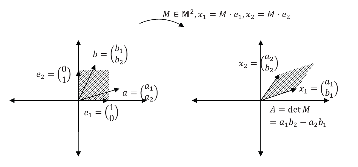
Let such that
![\[ M=\left(\begin{matrix}a_1 & a_2\\b_1& b_2\end{matrix}\right) \]](https://engcourses-uofa.ca/wp-content/ql-cache/quicklatex.com-2df76a619d07ddfe4e6ae17e45e8f8d6_l3.png "Rendered by QuickLaTeX.com")
The determinant of is defined as:
![\[ \det{M}=a_1b_2-a_2b_1 \]](https://engcourses-uofa.ca/wp-content/ql-cache/quicklatex.com-df219468f6d1dba4b6bd91ca1d28f7a2_l3.png "Rendered by QuickLaTeX.com")
Clearly, the vectors  and
and  are linearly dependent if and only if
  . The determinant of the matrix has a geometric meaning (See Figure 1). Consider the two unit vectors
  and
and  . Let
. Let  and
and  . The area of the parallelogram formed by and is equal to the determinant of the matrix .
The following is true  and
and  :
:
![\[\begin{split} \det{(NM)} & =\det{N}\det{M}\\ \det{\alpha M}& =\alpha^2\det{M}\\ \det{I} & = 1 \end{split} \]](https://engcourses-uofa.ca/wp-content/ql-cache/quicklatex.com-a5613454fceb3f0de7c24e15491488bc_l3.png "Rendered by QuickLaTeX.com")
where  is the identity matrix.

DETERMINANT OF  :
:
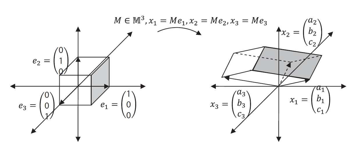
Let such that
![\[ M=\left(\begin{matrix}a_1 & a_2 & a_3\\b_1& b_2& b_3\\c_1&c_2&c_3\end{matrix}\right) \]](https://engcourses-uofa.ca/wp-content/ql-cache/quicklatex.com-4c2c270bf5cbca0ed8632a823160259d_l3.png "Rendered by QuickLaTeX.com")
If  , and
, and  , then the determinant of is defined as:
![\[ \det{M}=a\cdot (b\times c) \]](https://engcourses-uofa.ca/wp-content/ql-cache/quicklatex.com-7f7b6ca9752d98f6b0a6faddf80f54f2_l3.png "Rendered by QuickLaTeX.com")
I.e.,  the tripe product of
  , and
, and  . From the results of the triple product, the vectors , and are linearly dependent if and only if . The determinant of the matrix M has a geometric meaning (See Figure 2). Consider the three unit vectors
  , and
, and  . Let
. Let  , and
, and  . The determinant of is also equal to the triple product of
  , and
, and  and gives the volume of the parallelepiped formed by
  , and .
![\[\begin{split} \det{M}&=a\cdot(b\times c)=a_1(b_2c_3-b_3c_2)+a_2(b_3c_1-b_1c_3)+a_3(b_1c_2-b_2c_1)\\ &=a_1(b_2c_3-b_3c_2)+b_1(a_3c_2-a_2c_3)+c_1(a_2b_3-b_2a_3)\\ &=x_1\cdot (x_2\times x_3)\\ &=Me_1\cdot (Me_2\times Me_3) \end{split} \]](https://engcourses-uofa.ca/wp-content/ql-cache/quicklatex.com-d54db71ce4c372dd403eb18b02fdd2e9_l3.png "Rendered by QuickLaTeX.com")
Additionally,  and
and  are linearly independent, it is straightforward to show the following:
![\[ \det{M}=\frac{Mu\cdot(Mv\times Mw)}{u\cdot (v\times w)} \]](https://engcourses-uofa.ca/wp-content/ql-cache/quicklatex.com-71e5d09c2c7f24bc1c5072ed8dcc38c6_l3.png "Rendered by QuickLaTeX.com")
In other words, the determinant gives the ratio between  and
and  where is the volume of the transformed parallelepiped between
  , and
, and  and is the volume of the parallelepiped between
  , and
, and  .
The alternator
.
The alternator  defined in Mathematical Preliminaries can be used to write the followign useful equality:
![\[ \det{M}=Me_1\cdot(Me_2\times Me_3)\Rightarrow Me_i\cdot(Me_j\times Me_k)=\varepsilon_{ijk} \det{M} \]](https://engcourses-uofa.ca/wp-content/ql-cache/quicklatex.com-fbaad684dc4bf73238e60c42bb0ae1b0_l3.png "Rendered by QuickLaTeX.com")
The following is true  and :
and :
![\[\begin{split} \det{(NM)} & =\det{N}\det{M}\\ \det{\alpha M}& =\alpha^3\det{M}\\ \det{I} & = 1 \end{split} \]](https://engcourses-uofa.ca/wp-content/ql-cache/quicklatex.com-bc7c79cf72ab376ba7ccf41d74cd46db_l3.png "Rendered by QuickLaTeX.com")
where  is the identity matrix.

AREA TRANSFORMATION IN  :
:
The following is a very important formula (often referred to as “Nanson’s Formula”) that relates the cross product of vectors in to the cross product of their images under a linear transformation. This formula is used to relate area vectors before mapping to area vectors after mapping.
ASSERTION:
Let . Let be an invertible matrix. Show the following relationship:
![\[ Mu\times Mv = (\det{M})M^{-T}\left(u\times v\right) \]](https://engcourses-uofa.ca/wp-content/ql-cache/quicklatex.com-5a165eeb12e57e3f5383b8f1bccdbc2c_l3.png "Rendered by QuickLaTeX.com")
PROOF:
Let be an arbitrary vector in . From the relationships above we have:
![\[ Mw\cdot \left(Mu\times Mv\right)=(\det{M}) w\cdot (u\times v) \]](https://engcourses-uofa.ca/wp-content/ql-cache/quicklatex.com-e2751b4064c2b16ef795e68e644bbdde_l3.png "Rendered by QuickLaTeX.com")
Therefore:
![\[ w\cdot M^T\left(Mu\times Mv\right)=(\det{M}) w\cdot (u\times v) \]](https://engcourses-uofa.ca/wp-content/ql-cache/quicklatex.com-252bd41bedb35dbc16198ad345b94638_l3.png "Rendered by QuickLaTeX.com")
is arbitrary, it is straightforward to show that the vectors  and
and  are equal. And, since is invertible, so, is
  .
.
Therefore:
Nanson’s formula is sometimes written as follows:
![\[ a n = (\det{M})M^{-T}\left(A N\right) \]](https://engcourses-uofa.ca/wp-content/ql-cache/quicklatex.com-62a9f3d7d3fcdf095cf1e983d51f4747_l3.png "Rendered by QuickLaTeX.com")
where
![\[\begin{split} A&=\|u\times v\|\\ N&=\frac{1}{A}(u\times v)\\ a&=\|Mu\times Mv\|\\ n&=\frac{1}{a}(Mu\times Mv) \end{split} \]](https://engcourses-uofa.ca/wp-content/ql-cache/quicklatex.com-bad3133d928efed838a55b6f4b0b61ac_l3.png "Rendered by QuickLaTeX.com")
DETERMINANT OF :
The determinant of is defined using the recursive relationship:
![\[ \det{M}=\sum_{i=1}^n(-1)^{(i+1)}M_{1i}\det{N_i} \]](https://engcourses-uofa.ca/wp-content/ql-cache/quicklatex.com-b98962de31dcf9a29a7f038d262565a8_l3.png "Rendered by QuickLaTeX.com")
where  and is formed by eliminating the 1st row and column of the matrix . It can be shown that
  the rows of are linearly dependent.
Video
See “Area Transformation” Video here
Eigenvalues and Eigenvectors
Let  is called an eigenvalue of the tensor if
  such that
  . In this case,
  is called an eigenvector of associated with the eigenvalue
  .
.
Similar Matrices
Let  . Let be an invertible tensor. The matrix representations of the tensors and
  are termed “similar matrices”.
Similar matrices have the same eigenvalues while their eigenvectors differ by a linear transformation as follows: If  is an eigenvalue of with the associated eigenvector then:
![\[ Mp=\lambda p\Rightarrow MT^{-1}Tp=\lambda T^{-1}Tp\Rightarrow TMT^{-1}(Tp)=\lambda (Tp) \]](https://engcourses-uofa.ca/wp-content/ql-cache/quicklatex.com-cbc9f84c126c153f4539c1579650eb04_l3.png "Rendered by QuickLaTeX.com")
Therefore, is an eigenvalue of and  is the associated eigenvector. Similarly, if is an eigenvalue of with the associated eigenvector
  then:
then:
![\[ TMT^{-1}q=\lambda q\Rightarrow MT^{-1}q=\lambda T^{-1}q\Rightarrow M(T^{-1}q)=\lambda (T^{-1}q) \]](https://engcourses-uofa.ca/wp-content/ql-cache/quicklatex.com-c7aaccc014a29dc9216f9cdb07b85efe_l3.png "Rendered by QuickLaTeX.com")
Therefore, is an eigenvalue of and  is the associated eigenvector. Therefore, similar matrices share the same eigenvalues.
The Eigenvalues and Eigenvector Problem
Given a tensor , we seek a nonzero vector  and a real number such that: . This is equivalent to
  . In other words, the eigenvalue is a real number that makes the tensor
  not invertible while the eigenvector is a non-zero vector
  . Considering the matrix representation of the tensor , the eigenvalue is the solution to the following equation:
![\[ \det(M-\lambda I)=0 \]](https://engcourses-uofa.ca/wp-content/ql-cache/quicklatex.com-2356360275a1bc349b04f8c58f95c79a_l3.png "Rendered by QuickLaTeX.com")
The above equation is called the characteristic equation of the matrix .
From the properties of the determinant function, the characteristic equation is an  degree polynomial of the unknown where is the dimension of the underlying space.
In particular,  , where
  are called the polynomial coefficients. Thus, the solution to the characteristic equation abides by the following facts from polynomial functions:
– Polynomial roots: A polynomial  has a root
  if
if  divides , i.e.,
  such that
  .
.
– The fundamental theorem of Algebra states that a polynomial of degree has complex roots that are not necessarily distinct.
– The Complex Conjugate Root Theorem states that If is a complex root of a polynomial with real coefficients, then the conjugate  is also a complex root.
Therefore, the eigenvalues can either be real or complex numbers. If one eigenvalue is a real number, then there exists a vector with real valued components that is an eigenvector of the tensor. Otherwise, the only eigenvectors are complex eigenvectors which are elements of finite dimensional linear spaces over the field of complex numbers.
Graphical Representation of the Eigenvalues and Eigenvectors
The eigenvectors of a tensor are those vectors that do not change their direction upon transformation with the tensor but their length is rather magnified or reduced by a factor . Notice that an eigenvalue can be negative (i.e., the transformed vector can have an opposite direction). Additionally, an eigenvalue can have the value of 0. In that case, the eigenvector is an element of the kernel of the tensor.
The following example illustrates this concept. Choose four entries for the matrix  and press evaluate.
The tool then draws 8 coloured vectors across the circle and their respective images across the ellipse. Use visual inspection to identify which vectors keep their original direction.
and press evaluate.
The tool then draws 8 coloured vectors across the circle and their respective images across the ellipse. Use visual inspection to identify which vectors keep their original direction.
The tool also finds at most two eigenvectors (if they exist) and draws them in black along with their opposite directions. A similar tool is available on the external MecsimCalc python app builder. Use the tool to investigate the eigenvalues and eigenvectors of the following matrices:
![\[ \left(\begin{array}{cc} 1& 0\\ 0&1\end{array}\right)\hspace{10mm}\left(\begin{array}{cc} 1& 1\\ 0&1\end{array}\right)\hspace{10mm}\left(\begin{array}{cc} 0.4& 0.7\\-0.7&0.2\end{array}\right) \hspace{10mm}\left(\begin{array}{cc} 1& 2\\5&1\end{array}\right) \]](https://engcourses-uofa.ca/wp-content/ql-cache/quicklatex.com-84084893537e64fc2800d6af043c43f2_l3.png "Rendered by QuickLaTeX.com")
After inspection, you should have noticed that every vector is an eigenvector for the identity matrix since  , i.e., possesses one eigenvalue which is 1 but all the vectors in are possible eigenvectors.
You should also have noticed that some matrices don’t have any real eigenvalues, i.e., none of the vectors keep their direction after transformation. This is the case for the matrix:
![\[ M=\left(\begin{array}{cc} 0.4& 0.7\\-0.7&0.2\end{array}\right) \]](https://engcourses-uofa.ca/wp-content/ql-cache/quicklatex.com-925f7fd6099886500cc1898dfd4f0ef2_l3.png "Rendered by QuickLaTeX.com")
Additionally, the matrix:
![\[ N=\left(\begin{array}{cc} 1& 1\\0&1\end{array}\right) \]](https://engcourses-uofa.ca/wp-content/ql-cache/quicklatex.com-a0c756da20058a85ac398888c7a9f76b_l3.png "Rendered by QuickLaTeX.com")
has only one eigenvalue while any vector which is a multiplier of
![\[ p=\left(\begin{array}{cc} 1\\0\end{array}\right) \]](https://engcourses-uofa.ca/wp-content/ql-cache/quicklatex.com-f7bbb355a4bb9d9df492fc524890bdd7_l3.png "Rendered by QuickLaTeX.com")
keeps its direction after transformation through the matrix . You should also notice that some matrices will have negative eigenvalues. In that case, the corresponding eigenvector will be transformed into the direction opposite to its original direction. See for example, the matrix:
![\[ O=\left(\begin{array}{cc} 1& 2\\5&1\end{array}\right) \]](https://engcourses-uofa.ca/wp-content/ql-cache/quicklatex.com-a93d999c97533fd4f97ddf532ca2ac00_l3.png "Rendered by QuickLaTeX.com")
Videos:
2.2.1 Basic Definitions
2.2.1.4 Tensor Product
Refer to this section.
2.2.1.7 Area Transformation
Refer to this section.
https://mecsimcalc.com/app/5787840/graphical_representation_of_the_eigenvalues_and_eigenvectors