
Plasticity: Examples and Problems
Examples
Example 1: Isotropic Hardening
The “true” stress versus “true” strain of a metallic material follows a bilinear relationship with true strains of 0.002 and 0.25 corresponding to stress levels of 400 and 550 MPa respectively. If Young’s modulus and Poisson’s ratio are equal to 200GPa and 0.3 respectively. Using von Mises incremental plasticity with isotropic hardening find the components of the elastic strain, the plastic strain and the total strain, the magnitude of the equivalent plastic strain parameter as a function of  . Evaluate the total strains at
  . Plot the relationship between and the total longitudinal strain component
  in each of the following conditions.
Condition 1: If a specimen is under a uniaxial state of stress.
Condition 2: If a specimen is under a stress
and  is kept at 0 in a plane stress condition.
Condition 3: If a specimen is under a stress
and is kept at 0 in a plane strain condition.
Solution
First, the relationship between  and
and  is obtained from the information given. At
  , the elastic strain
  while the plastic strain
  . At
. At  , the elastic strain
  while the plastic strain
  . Thus, the relationship between and the plastic strain parameter is as follows:
![\[\sigma_Y = 400 + 150\frac{\overline{\varepsilon^p}}{0.24725}\]](https://engcourses-uofa.ca/wp-content/ql-cache/quicklatex.com-3b7d717b2678c9c2eb48909eb1c1e5f6_l3.png "Rendered by QuickLaTeX.com")
The slope of this relationship is constant and can be calculated as follows:
![\[h = \frac{d\sigma_Y}{d \overline{\varepsilon^p}} = 606.673\]](https://engcourses-uofa.ca/wp-content/ql-cache/quicklatex.com-ecb0802598b2a08068e7ec22173e5bd5_l3.png "Rendered by QuickLaTeX.com")
Thus, the relationship between and the plastic strain parameter can be written as:
![\[\sigma_Y = 400 + h\overline{\varepsilon^p}\]](https://engcourses-uofa.ca/wp-content/ql-cache/quicklatex.com-05526b19e354c20a5d257ed666f446b4_l3.png "Rendered by QuickLaTeX.com")
Condition 1: Uniaxial State of Stress
In a uniaxial state of stress condition, the hydrostatic stress, the von Mises stress, the Cauchy stress the deviatoric stress matrices have the following forms:
![\[p = \frac{\sigma_{11}}{3} \hspace{5mm} \sigma_{vM} = \sigma_{11} \hspace{5mm} \sigma = \begin{pmatrix} \sigma_{11} & 0 & 0 \\ 0 & 0 & 0 \\ 0 & 0 & 0 \\ \end{pmatrix} \hspace{5mm} S = \begin{pmatrix} \frac{2 \sigma_{11}}{3} & 0 & 0 \\ 0 & -\frac{\sigma_{11}}{3} & 0 \\ 0 & 0 & -\frac{\sigma_{11}}{3} \\ \end{pmatrix}\]](https://engcourses-uofa.ca/wp-content/ql-cache/quicklatex.com-95191a482e21530e3cc5ffbab8b1930c_l3.png "Rendered by QuickLaTeX.com")
The elastic strain components can be obtained using the elastic constitutive relationships as follows:
![\[\varepsilon_{11}^e = \frac{\sigma_{11}}{E} \hspace{5mm} \varepsilon_{22}^e = \varepsilon_{33}^3 = -\nu \frac{\sigma_{11}}{E} \hspace{5mm} \varepsilon_{12}^e = \varepsilon_{13}^e = \varepsilon_{23}^e = 0\]](https://engcourses-uofa.ca/wp-content/ql-cache/quicklatex.com-ad958e745092b5c321b6959f840f76d2_l3.png "Rendered by QuickLaTeX.com")
The plastic strain components can be obtained as follows:
When  ,
,  and the total strain components are equal to the elastic strain components.
When  , the increment in the plastic strain parameter
  can be obtained from the consistency condition:
![\[d\phi = 0 \approx \Delta \phi = \frac{\partial \sigma_{vM}}{\partial \sigma_{ij}} \Delta \sigma_{ij} - \frac{d\sigma_Y}{d \overline{\varepsilon^p}} \Delta \overline{\varepsilon^p} = \frac{3S_{11}}{2\sigma_{vM}} \Delta \sigma_{11} - h \Delta \overline{\varepsilon^p} = \Delta \sigma_{11} - h \Delta \overline{\varepsilon^p}\]](https://engcourses-uofa.ca/wp-content/ql-cache/quicklatex.com-343ea4499e122ced237b77af8ae79cdb_l3.png "Rendered by QuickLaTeX.com")
Thus, an increment  will produce an increment in the plastic strain parameter
  that is equal to:
![\[\Delta \overline{\varepsilon^p} = \frac{\Delta \sigma_{11}}{h}\]](https://engcourses-uofa.ca/wp-content/ql-cache/quicklatex.com-ce489b2f2242f451dba3418f4f943a53_l3.png "Rendered by QuickLaTeX.com")
The magnitude of the plastic strain parameter can be obtained by summing (or integrating) the increments as follows:
![\[\overline{\varepsilon^p} = \int_{400}^{\sigma_{11}} \frac{1}{h} d\sigma_{11} = \frac{\sigma_{11} - 400}{h}\]](https://engcourses-uofa.ca/wp-content/ql-cache/quicklatex.com-afa3f8b6204531c3c1b438507d86f125_l3.png "Rendered by QuickLaTeX.com")
The increments in the plastic strain components can be obtained as follows:
![\[\Delta \varepsilon_{ij}^p = \Delta \overline{\varepsilon^p} \frac{\partial \phi}{\partial \sigma_{ij}} = \Delta \overline{\varepsilon^p} \frac{3S_{ij}}{2\sigma_{vM}}\]](https://engcourses-uofa.ca/wp-content/ql-cache/quicklatex.com-47d737b95729f7d55729393e5d8ee1de_l3.png "Rendered by QuickLaTeX.com")
Thus:
![\[\Delta \varepsilon_{11}^p = \Delta \overline{\varepsilon^p} \hspace{5mm} \Delta \varepsilon_{22}^p = \Delta \varepsilon_{33}^p = -\frac{\Delta \overline{\varepsilon^p}}{2} \hspace{5mm} \Delta \varepsilon_{12}^p = \Delta \varepsilon_{13}^p = \Delta \varepsilon_{23}^p = 0\]](https://engcourses-uofa.ca/wp-content/ql-cache/quicklatex.com-142fbc1aa85b60b8561fce5f35d2c77c_l3.png "Rendered by QuickLaTeX.com")
The plastic strain components are equal to the sum of the respective increments and since  is constant for this particular material and there is no unloading:
![\[\varepsilon_{11}^p = \int_{400}^{\sigma_{11}} \frac{1}{h} d\sigma_{11} = \frac{\sigma_{11} - 400}{h} \hspace{5mm} \varepsilon_{22}^p = \varepsilon_{33}^p = -\frac{\varepsilon_{11}^p}{2}\]](https://engcourses-uofa.ca/wp-content/ql-cache/quicklatex.com-5a02386b3b236263a41da8f217ef2746_l3.png "Rendered by QuickLaTeX.com")
The total strains at a stress level  are obtained as:
![\[\varepsilon_{11} = \varepsilon_{11}^e +\varepsilon_{11}^p = \frac{\sigma_{11}}{E} + \frac{\sigma_{11} - 400}{h}\]](https://engcourses-uofa.ca/wp-content/ql-cache/quicklatex.com-2157d1f94a8d583b54c9d9a754948bfc_l3.png "Rendered by QuickLaTeX.com")
![\[\varepsilon_{22} = \varepsilon_{33} = \varepsilon_{22}^e + \varepsilon_{22}^p = -\nu \frac{\sigma_{11}}{E} - \frac{\sigma_{11}-400}{2h}\]](https://engcourses-uofa.ca/wp-content/ql-cache/quicklatex.com-0793e12608e4578e5345815fbdea2601_l3.png "Rendered by QuickLaTeX.com")
![\[\varepsilon_{12} = \varepsilon_{13} = \varepsilon_{23} = 0\]](https://engcourses-uofa.ca/wp-content/ql-cache/quicklatex.com-65b809a4b36946169b5aac7678282eed_l3.png "Rendered by QuickLaTeX.com")
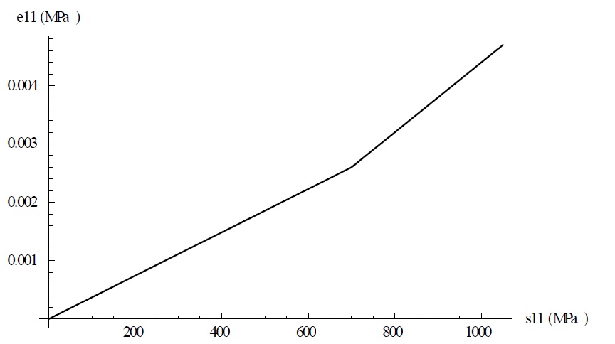
Notice that the relationship between and the total strain follows that given by the material curve:
![\[\varepsilon_{11} = \begin{cases} \frac{\sigma_{11}}{E} & \sigma_{11} \le 400 \\ \frac{\sigma_{11}}{E} + \frac{\sigma_{11}-400}{h} & \sigma_{11} > 400 \\ \end{cases} \Rightarrow \sigma_{11} = \begin{cases} E \varepsilon_{11} & \varepsilon_{11} \le 0.002 \\ \frac{E(400+h\varepsilon_{11})}{E+h} & \varepsilon_{11} > 0.002 \\ \end{cases}\]](https://engcourses-uofa.ca/wp-content/ql-cache/quicklatex.com-9bf73389a5b239451a9417c675940d33_l3.png "Rendered by QuickLaTeX.com")
Condition 2: Plane Stress Condition with 
The Cauchy stress and the deviatoric stress matrices have the following forms:
![\[\sigma = \begin{pmatrix} \sigma_{11} & 0 & 0 \\ 0 & \sigma_{22} & 0 \\ 0 & 0 & 0 \\ \end{pmatrix} \hspace{5mm} S = \begin{pmatrix} \frac{2\sigma_{11} - \sigma_{22}}{3} & 0 & 0 \\ 0 & \frac{2\sigma_{22} - \sigma_{11}}{3} & 0 \\ 0 & 0 & \frac{-\sigma_{11} - \sigma_{22}}{3} \\ \end{pmatrix}\]](https://engcourses-uofa.ca/wp-content/ql-cache/quicklatex.com-fec371dd5106bf75e03390388277a7f3_l3.png "Rendered by QuickLaTeX.com")
In this case, the onset of initial yielding occurs when  , i.e., when:
![\[\sigma_{11}^2 - \sigma_{11}\sigma_{22} + \sigma_{22}^2 = (400)^2\]](https://engcourses-uofa.ca/wp-content/ql-cache/quicklatex.com-dd6afab5253c1324b79aae5d5644f23a_l3.png "Rendered by QuickLaTeX.com")
Before developing any plastic strains, the total strain component is equal to the elastic strain component  . The condition of loading ensures that
  and thus:
![\[\varepsilon_{22}^e = \frac{\sigma_{22}}{E} - \frac{\nu \sigma_{11}}{E} = 0 \Rightarrow \sigma_{22} = \nu \sigma_{11}\]](https://engcourses-uofa.ca/wp-content/ql-cache/quicklatex.com-7847da8116647ff6b7ea859398108eff_l3.png "Rendered by QuickLaTeX.com")
Therefore, at the onset of initial yielding:
![\[\sigma_{11} = \frac{400}{\sqrt{1-\nu + \nu^2}} \approx 450MPa \hspace{5mm} \sigma_{22} = \frac{\nu 400}{\sqrt{1-\nu+ \nu^2}} \approx 135MPa\]](https://engcourses-uofa.ca/wp-content/ql-cache/quicklatex.com-5c9cca1e0313ff9f79fe6cc9fab1250d_l3.png "Rendered by QuickLaTeX.com")
Therefore, when  , the plastic strain components are zero while the elastic strain components are given by:
![\[\varepsilon_{11}^e = \frac{\sigma_{11}}{E} (1-\nu^2) \hspace{5mm} \varepsilon_{22}^e = 0 \hspace{5mm} \varepsilon_{33}^e = -\frac{\nu \sigma_{11}}{E} (1+\nu)\]](https://engcourses-uofa.ca/wp-content/ql-cache/quicklatex.com-ee816f0d8dc063c8976f2792378cf77d_l3.png "Rendered by QuickLaTeX.com")
Once yielding occurs, the relationship between the stress components obtained above no longer follows. We seek to find expressions of the evolution of the elastic and plastic strain components as a function of the changes in the stress component. To do that, we first note that there are two nonzero stress components in the stress matrix, these are and  . We also note that the condition of the total strain can be used to relate the rate of changes of the stress components together. However, the total strain component has elastic and plastic components. The plastic component is a function of the plastic strain parameter . So, the consistency condition is also used to relate the rates of the nonzero stress components with the rate of change of the plastic strain parameter. In other words, two equations are used to relate the rates of change of and of to the rate of change of . The following shows the details of the procedure here.
First, the consistency condition can be used to relate the rate of change of the equivalent plastic strain parameter to the rate of change of the stress components:
![\[\dot{\phi} = \dot{\sigma}_{vM} - \dot{\sigma}_{Y} = 0 \Rightarrow \frac{\partial \sigma_{vM}}{\partial \sigma_{ij}} \dot{\sigma}_{ij} - \frac{d\sigma_Y}{d\overline{\varepsilon^p}} \dot{\overline{\varepsilon^p}} = 0 \Rightarrow \frac{3S_{11}}{2\sigma_{vM}} \dot{\sigma}_{11} + \frac{3S_{22}}{2\sigma_{vM}} \dot{\sigma}_{22} - h\overline{\varepsilon^p} = 0\]](https://engcourses-uofa.ca/wp-content/ql-cache/quicklatex.com-e8cf78194976e9fa62d6cf3bea51b3b1_l3.png "Rendered by QuickLaTeX.com")
Rearranging yields the relationship between the rate of change of the equivalent plastic strain parameter and the rate of change of the stress components:
![\[\dot{\overline{\varepsilon^p}} = \frac{(2\sigma_{11} - \sigma_{22}) \dot{\sigma}_{11} + (2\sigma_{22} - \sigma_{11}) \dot{\sigma}_{22}} {2h\sigma_{vM}}\]](https://engcourses-uofa.ca/wp-content/ql-cache/quicklatex.com-0d39ac07d0326727894ade9395fe55e7_l3.png "Rendered by QuickLaTeX.com")
The boundary conditions dictate that  , which leads to the following relationship between the rates of the equivalent plastic strain and the stress components:
![\[\frac{\dot{\sigma}_{22}}{E} - \frac{\nu \dot{\sigma}_{11}}{E} + \dot{\overline{\varepsilon^p}} \frac{\partial \phi}{\partial \sigma_{22}} = 0\]](https://engcourses-uofa.ca/wp-content/ql-cache/quicklatex.com-c41be22b0da02b8296f98be060285034_l3.png "Rendered by QuickLaTeX.com")
Substituting for  in the above equation yields
  as an explicit function of
  , and :
![\[\dot{\sigma}_{22} = \dot{\sigma}_{11} \frac{E(\sigma_{11} - 2\sigma_{22})(2\sigma_{11}-\sigma_{22}) + 4h\nu \sigma_{vM}^2}{E(\sigma_{11} - 2\sigma_{22})^2 + 4h\sigma_{vM}^2}\]](https://engcourses-uofa.ca/wp-content/ql-cache/quicklatex.com-6220fa24d1d6c100842941cd4b5fda60_l3.png "Rendered by QuickLaTeX.com")
Substituting the value of back into the expression of yields the following:
![\[\dot{\overline{\varepsilon^p}} = 2\dot{\sigma}_{11} \frac{((2 - \nu)\sigma_{11} + \sigma_{22}(2\nu - 1))\sigma_{vM}} {E(\sigma_{11} - 2\sigma_{22})^2 + 4h\sigma_{vM}^2}\]](https://engcourses-uofa.ca/wp-content/ql-cache/quicklatex.com-c24daae8f8989c73174112b2b0a3cd79_l3.png "Rendered by QuickLaTeX.com")
The rate of change of the individual plastic strain components can then be calculated as a function of as follows:
![\[\dot{\varepsilon}_{ij}^p = \dot{\overline{\varepsilon^p}} \frac{\partial \phi}{\partial \sigma_{ij}} = \dot{\overline{\varepsilon^p}} \frac{3S_{ij}}{2\sigma_{vM}}\]](https://engcourses-uofa.ca/wp-content/ql-cache/quicklatex.com-0f605cc42d1a2b743e1265166f3521e5_l3.png "Rendered by QuickLaTeX.com")
Substituting for , the following expressions are obtained:
![\[\dot{\varepsilon}_{11}^p = \dot{\sigma_{11}}(2\sigma_{11}-\sigma_{22}) \frac{\sigma_{11}(2-\nu) + \sigma_{22}(2\nu - 1)}{E(\sigma_{11}-2\sigma_{22})^2 + 4h\sigma_{vM}^2}\]](https://engcourses-uofa.ca/wp-content/ql-cache/quicklatex.com-6ebc7d05c5782118eb1b57cf47629fc7_l3.png "Rendered by QuickLaTeX.com")
![\[\dot{\varepsilon}_{22}^p = \dot{\sigma_{11}}(2\sigma_{22}-\sigma_{11}) \frac{\sigma_{11}(2-\nu) + \sigma_{22}(2\nu - 1)}{E(\sigma_{11}-2\sigma_{22})^2 + 4h\sigma_{vM}^2}\]](https://engcourses-uofa.ca/wp-content/ql-cache/quicklatex.com-b06d228cfbdb4b75db1258aa12ee997f_l3.png "Rendered by QuickLaTeX.com")
![\[\dot{\varepsilon}_{33}^p = \dot{\sigma_{11}}(\sigma_{11}+\sigma_{22}) \frac{\sigma_{11}(\nu -2) + \sigma_{22}(1 - 2\nu)}{E(\sigma_{11}-2\sigma_{22})^2 + 4h\sigma_{vM}^2}\]](https://engcourses-uofa.ca/wp-content/ql-cache/quicklatex.com-20e307acfa2e094771aa7fd1900320a9_l3.png "Rendered by QuickLaTeX.com")
The problem reduces to finding a solution to the ordinary differential equations of the following form:
![\[\dot{\sigma}_{22} = f(\sigma_{11}, \sigma_{22}, \dot{\sigma}_{11}) \hspace{5mm} \dot{\overline{\varepsilon^p}} = g(\sigma_{11}, \sigma_{22}, \dot{\sigma}_{11}) \hspace{5mm} \dot{\varepsilon}_{ij}^p = h_{ij}(\sigma_{11}, \sigma_{22}, \dot{\sigma}_{11})\]](https://engcourses-uofa.ca/wp-content/ql-cache/quicklatex.com-aa7bcaaffa3929383a7637cecb6fa608_l3.png "Rendered by QuickLaTeX.com")
The initial conditions for these equations are given by  ,
,  ,
,  . The rate of change of , namely can be arbitrarily chosen. In order to solve the above ordinary differential equations, an independent time parameter t is introduced such that
  , therefore,
  . The integration of the above equations can be performed numerically using a spreadsheet or using the NDSolve[] function in Mathematica with an arbitrary upper limit for or
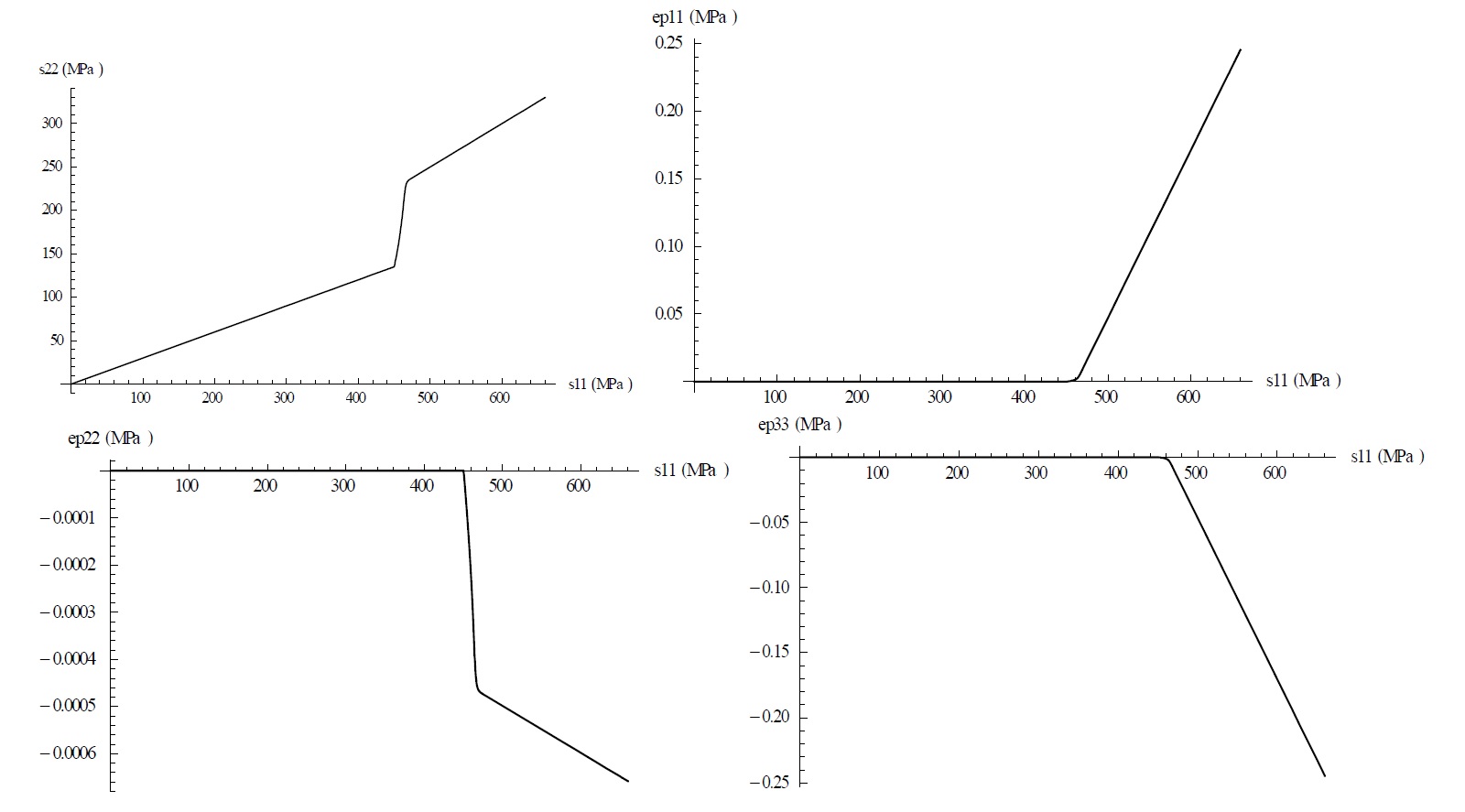
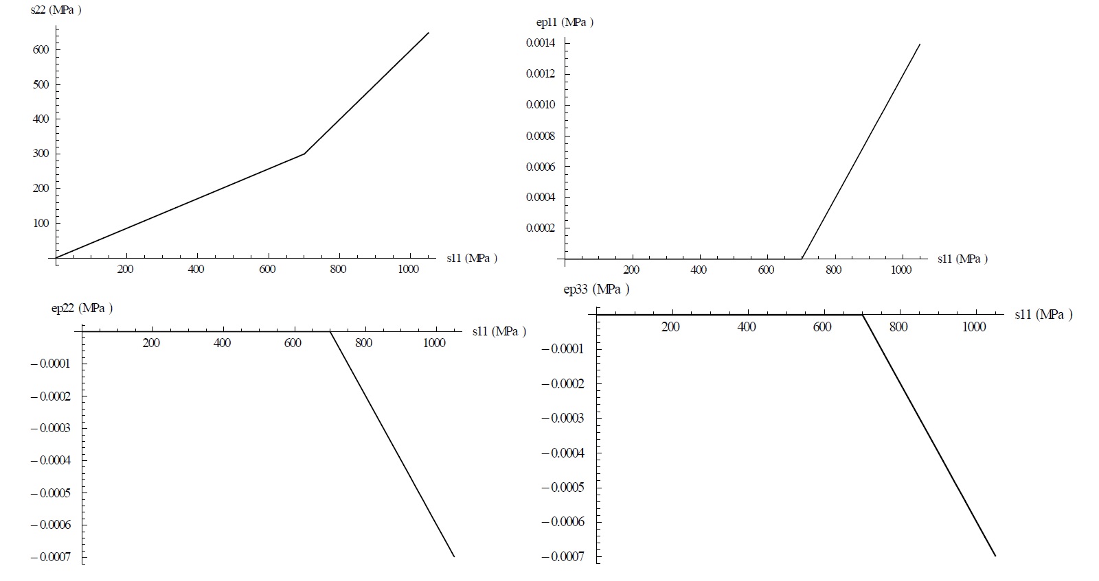
  , which in this example was taken as 650MPa. Note that if a spreadsheet is to be used, then the backward Euler integration method would produce more accurate results than the forward Euler integration method.
The following figures show the plots of and the various nonzero plastic strain components as a function of . The plot of versus reveals three different regions during the loading process. In the initial elastic region, the stresses are related using Poisson’s ratio. In the second region, as plastic strain develops, the stress increases rapidly up to around half . In the third region, as increases, the stress is almost half that of . The plastic strain components reveal that as the specimen is pulled beyond its initial elasticity limit, positive
, which in this example was taken as 650MPa. Note that if a spreadsheet is to be used, then the backward Euler integration method would produce more accurate results than the forward Euler integration method.
The following figures show the plots of and the various nonzero plastic strain components as a function of . The plot of versus reveals three different regions during the loading process. In the initial elastic region, the stresses are related using Poisson’s ratio. In the second region, as plastic strain develops, the stress increases rapidly up to around half . In the third region, as increases, the stress is almost half that of . The plastic strain components reveal that as the specimen is pulled beyond its initial elasticity limit, positive  strain is developed. In contract, negative
  and
and  are developed. This indicates that if the stresses are removed, the specimen will be longer in the direction of the basis vector
  while shorter in the other two directions. The sum of the plastic strain components
  is always equal to zero.
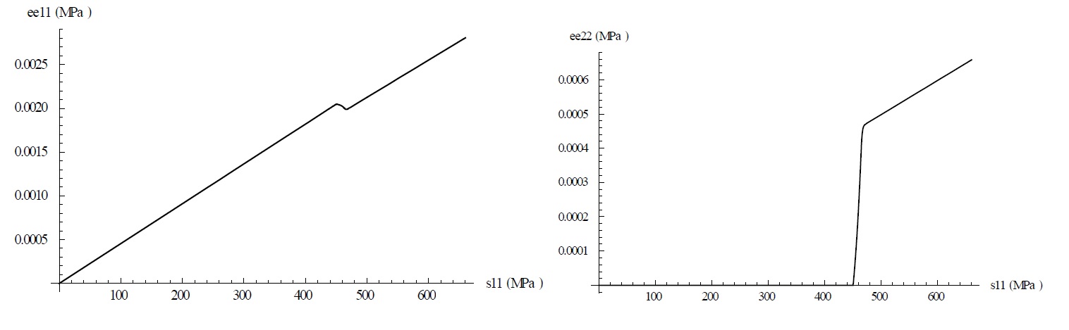
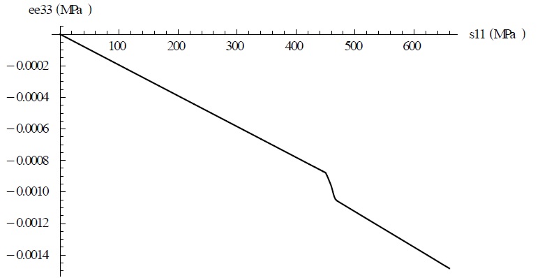
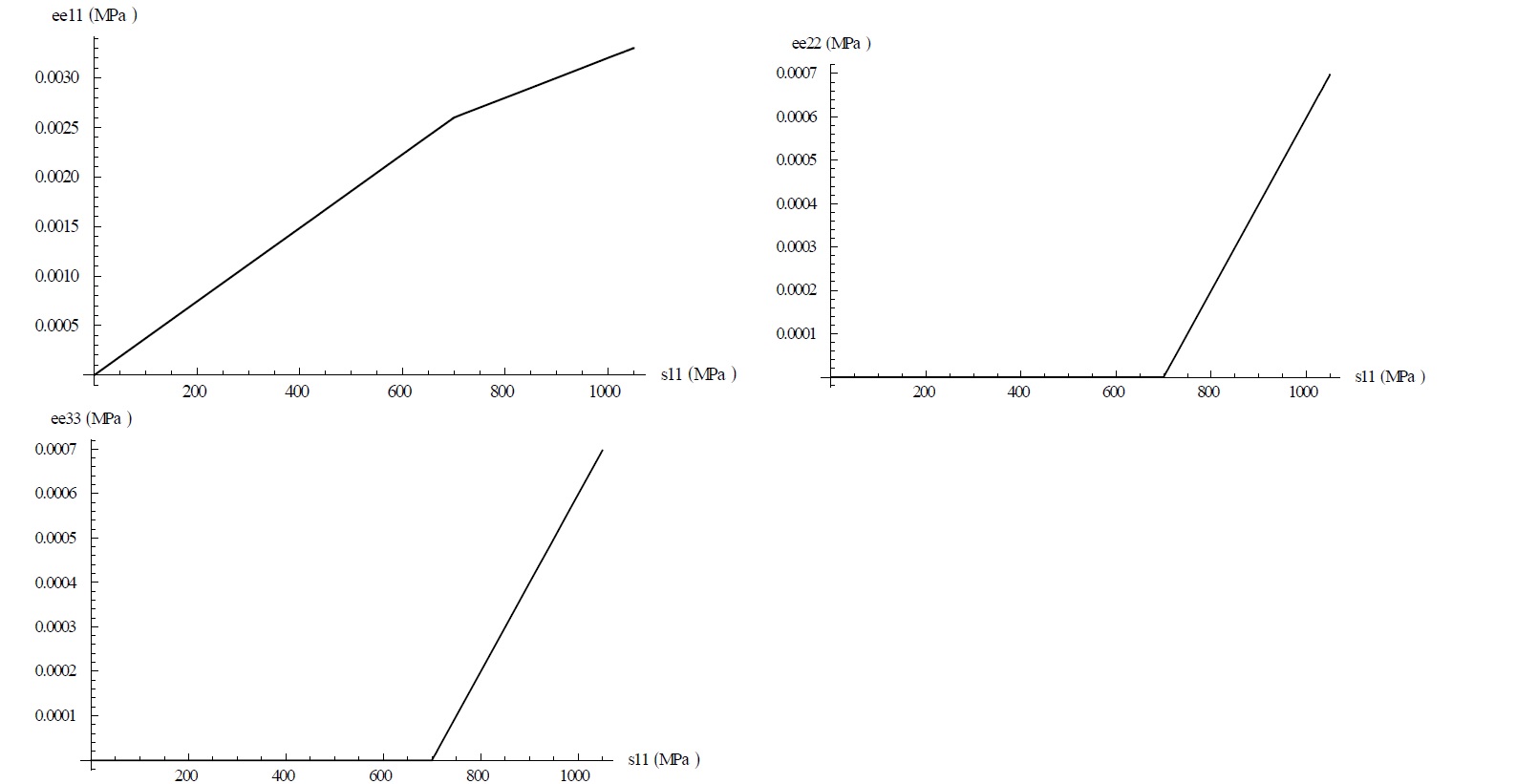
The following figures show the plots of the various nonzero elastic strain components as a function of . Notice that the elastic strain is equal to zero when is less than the initial elastic limit. Beyond that, increases rapidly similar to the plastic strain component but with a negative sign to maintain a zero value for the total strain .
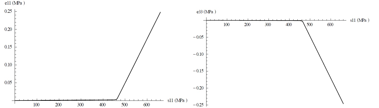
The following figures show the plots of the various nonzero total strain components as a function of :
View Mathematica Code
Clear[ds11,ds22,Svm,s11,s22,s33]
(*Values of material constants*)
epmax=25/100-550/200000;
hslope=N[150/epmax];
rule={Ee->200000,nu->0.3,h->hslope};
(*Stress, hydrostatic stress, deviatoric stress and von Mises stress*)
s={{s11,0,0},{0,s22,0},{0,0,s33}};
hydr=(s11+s22+s33)/3;
s33=0;
Sdev=FullSimplify[s-hydr*IdentityMatrix[3]];
Sdev//MatrixForm
Sigmavm=Sqrt[1/2*((s11-s22)^2+(s11-s33)^2+(s22-s33)^2)];
s=FullSimplify[(Sigmavm)^2]
(*The stresses at the elastic limit utilizing ee22=0*)
b=Solve[{Sqrt[s]==sys,s22==nu*s11},{s11,s22}]
(*The strains at the elastic limit*)
ee11=(s11/Ee-nu*s22/Ee)/.s22->nu*s11
ee22=(-nu*s11/Ee+s22/Ee)/.s22->nu*s11
ee33=(-nu*s11/Ee-nu*s22/Ee)/.s22->nu*s11
Sdev=Sdev/.{s11->s11[t],s22->s22[t]}
Sigmavm=Sigmavm/.{s11->s11[t],s22->s22[t]}
(*Consistency condition*)
cep'[t]=(3/2*Sdev[[1,1]]*s11'[t]/h/Svm+3/2*Sdev[[2,2]]*s22'[t]/h/Svm)
(*ep22 Plastic strain Rate *)
cep22'[t]=FullSimplify[cep'[t]*3/2*Sdev[[2,2]]/Svm]
(*ee22 elastic strain rate*)
Clear[ee22]
ee22'[t]=s22'[t]/Ee-nu*s11'[t]/Ee
(*Finding the relationship between s11'[t] and s22'[t]*)
a=FullSimplify[Solve[ee22'[t]+cep22'[t]==0,{s22'[t]}]]
(*Making everything function of s11'[t] alone*)
eq1=ep'[t]==FullSimplify[cep'[t]/.a[[1]]]
eq2=ep11'[t]==FullSimplify[(cep'[t]/.a[[1]])*3/2*Sdev[[1,1]]/Svm]
eq3=ep22'[t]==FullSimplify[(cep'[t]/.a[[1]])*3/2*Sdev[[2,2]]/Svm]
eq4=ep33'[t]==FullSimplify[(cep'[t]/.a[[1]])*3/2*Sdev[[3,3]]/Svm]
(*Finding s11 and s22 as a function of t using NDsolve, the procedure  assumes s11=t*)
s22equation=s22'[t]/.a[[1]]
s22equation=s22equation/.rule;
Svm=Sigmavm/.rule;
s11initial=400/Sqrt[1-nu+nu^2]/.rule;
ff=NDSolve[{(s22'[t]==s22equation),s11'[t]==1,s11[s11initial]==s11initial,
(s22[s11initial]==(nu/.rule)*s11initial)},{s22,s11},{t,s11initial,650}]
s22function=Piecewise[{{nu*t/.rule,0<=t<=s11initial},{s22[t]/.ff[[1]],t>s11initial}}]
(*Finding plastic strain components as a function of t using NDsolve, the procedure assumes s11=t*)
rule2={s11[t]->t,s22[t]->s22function,s22'[t]->D[s22function,t],s11'[t]->1};
crule=Flatten[{rule,rule2}]
eq1=eq1/.crule
eq2=eq2/.crule;
eq3=eq3/.crule;
eq4=eq4/.crule;
a=NDSolve[{eq1,ep[s11initial]==0},ep,{t,s11initial,650}]
b=NDSolve[{eq2,ep11[s11initial]==0},ep11,{t,s11initial,650}]
c=NDSolve[{eq3,ep22[s11initial]==0},ep22,{t,s11initial,650}]
d=NDSolve[{eq4,ep33[s11initial]==0},ep33,{t,s11initial,650}]
(*Plastic Strain functions of s11=t*)
epfunction=Piecewise[{{0,0<=t<=s11initial},{ep[t]/.a[[1]],t>s11initial}}]
ep11function=Piecewise[{{0,0<=t<=s11initial},{ep11[t]/.b[[1]],t>s11initial}}]
ep22function=Piecewise[{{0,0<=t<=s11initial},{ep22[t]/.c[[1]],t>s11initial}}]
ep33function=Piecewise[{{0,0<=t<=s11initial},{ep33[t]/.d[[1]],t>s11initial}}]
(*Elastic Strain functions of s11=t and s22*)
ee11function=(t/Ee-s22function/Ee*nu)/.rule;
ee22function=(-nu*t/Ee+s22function/Ee)/.rule;
ee33function=(-nu*t/Ee-nu*s22function/Ee)/.rule;
(*Producing the plots*)
Plot[s22function,{t,0,660},PlotRange->All,AxesOrigin->{0,0},AxesLabel->{"s11(MPa)","s22(MPa)"},PlotStyle->Black]
Plot[ep11function,{t,0,660},PlotRange->All,AxesOrigin->{0,0},AxesLabel->{"s11(MPa)","ep11(MPa)"},PlotStyle->Black]
Plot[ep22function,{t,0,660},PlotRange->All,AxesOrigin->{0,0},AxesLabel->{"s11(MPa)","ep22(MPa)"},PlotStyle->Black]
Plot[ep33function,{t,0,660},PlotRange->All,AxesOrigin->{0,0},AxesLabel->{"s11(MPa)","ep33(MPa)"},PlotStyle->Black]
Plot[epfunction,{t,0,660},PlotRange->All,AxesOrigin->{0,0},AxesLabel->{"s11(MPa)","ep(MPa)"},PlotStyle->Black]
Plot[ee11function,{t,0,660},PlotRange->All,AxesOrigin->{0,0},AxesLabel->{"s11(MPa)","ee11(MPa)"},PlotStyle->Black]
Plot[ee22function,{t,0,660},PlotRange->All,AxesOrigin->{0,0},AxesLabel->{"s11(MPa)","ee22(MPa)"},PlotStyle->Black]
Plot[ee33function,{t,0,660},PlotRange->All,AxesOrigin->{0,0},AxesLabel->{"s11(MPa)","ee33(MPa)"},PlotStyle->Black]
Plot[ee11function+ep11function,{t,0,660},PlotRange->All,AxesOrigin->{0,0},AxesLabel->{"s11(MPa)","e11(MPa)"},PlotStyle->Black]
Plot[Chop[ee22function+ep22function,10^-7],{t,0,660},PlotRange->All,AxesOrigin->{0,0},AxesLabel->{"s11(MPa)","e22(MPa)"},PlotStyle->Black]
Plot[ee33function+ep33function,{t,0,660},PlotRange->All,AxesOrigin->{0,0},AxesLabel->{"s11(MPa)","e33(MPa)"},PlotStyle->Black]
View Python Code
from sympy import *
import sympy as sp
import numpy as np
import matplotlib.pyplot as plt
from scipy.integrate import odeint
from scipy.interpolate import InterpolatedUnivariateSpline
sp.init_printing(use_latex = "mathjax")
s11, s22, nu, E, h, Svm, t = symbols("\u03c3_{11} \u03c3_{22} nu E h \u03c3_{vM} t")
epmax = 25/100-550/200000
hslope = 150/epmax
display(epmax)
display(hslope)
rule = {E:200000, nu:0.3, h:hslope}
display("Stress, hydrostatic stress, deviatoric stress and von Mises stress")
s33 = 0
s = Matrix([[s11,0,0],[0,s22,0],[0,0,s33]])
hydr = (s11+s22+s33)/3
display("Cauchy stress: ", s)
Sdev = s-hydr*eye(3)
display("Deviatoric stress: ", Sdev)
Sigmavn = sqrt(1/2*((s11-s22)**2+(s11-s33)**2+(s22-s33)**2))
s = simplify(Sigmavn**2)
display(s)
display("The stresses at the elastic limit utilizing ee22=0")
b = solve((sqrt(s) - 400, s22 - s11*nu), (s11,s22))
display(b)
display("The strains at the elastic limit")
ee11=(s11/E-nu*s22/E).subs(s22,nu*s11)
ee22=(-nu*s11/E+s22/E).subs(s22,nu*s11)
ee33=(-nu*s11/E-nu*s22/E).subs(s22,nu*s11)
display(ee11,ee22,ee33)
s11t = Function('\u03c3_{11}')
s22t = Function('\u03c3_{22}')
Sdev = Sdev.subs({s11:s11t(t), s22:s22t(t)})
Sigmavn = Sigmavn.subs({s11:s11t(t), s22:s22t(t)})
display("Consistency condition")
display(Sdev)
ceptp = (3/2*Sdev[0,0]*s11t(t).diff(t)/h/Svm+3/2*Sdev[1,1]*s22t(t).diff(t)/h/Svm)
display(ceptp)
display("ep22 Plastic strain Rate")
cep22tp = simplify(ceptp*3/2*Sdev[1,1]/Svm)
display(cep22tp)
display("ee22 Elastic strain Rate")
ee22tp = s22t(t).diff(t)/E-nu*s11t(t).diff(t)/E
display(ee22tp)
display("Finding the relationship between s11t and s22t")
a = solve(ee22tp + cep22tp, s22t(t).diff(t))
display(a)
display("Making everything a function of s11t alone")
eq1 = eptp = simplify(ceptp.subs(s22t(t).diff(t), a[0]))
eq2 = ep11tp = simplify(ceptp.subs(s22t(t).diff(t), a[0])*3/2*Sdev[0,0]/Svm)
eq3 = ep22tp = simplify(ceptp.subs(s22t(t).diff(t), a[0])*3/2*Sdev[1,1]/Svm)
eq4 = ep33tp = simplify(ceptp.subs(s22t(t).diff(t), a[0])*3/2*Sdev[2,2]/Svm)
display(eq1, eq2, eq3, eq4)
display("Finding s11 and s22 as a function of t using NDsolve, the procedure  assumes s11=t")
s22equation = a[0].subs(rule)
Svmsubs = Sigmavn.subs(rule)
s11initial = (400/sqrt(1-nu+nu**2)).subs(rule)
display(s22equation, Svmsubs, s11initial)
s22equation = s22equation.subs(Svm,Svmsubs)
s22equ = s22equation.subs({s11t(t):s11, s22t(t):s22, s11t(t).diff(t):1})
def rhs1(y,t):
    f = sp.lambdify([s11, s22], s22equ)
    f = f(y[0],y[1])
    ds22tdt = f
    dss11tdt = 1
    return [dss11tdt,ds22tdt]
s11initial = float(s11initial)
t1 = np.linspace(s11initial,650,20)
s22t0 = nu.subs(rule)*s11initial
s11t0 = s11initial
yzero = [s11t0,s22t0]
ff = odeint(rhs1, yzero, t1)
# display(ff)
# plot results
# aa is for plot1
lambda1 = lambda t : t*nu.subs(rule)
xL = np.linspace(0,s11initial,2)
fig, ax = plt.subplots(6,2, figsize = (20,30))
plt.setp(ax[0,0], xlabel = "s11", ylabel = "s22")
ax[0,0].plot(ff[:,0],ff[:,1],'b-')
ax[0,0].plot(xL,lambda1(xL),'b-')
def integralsolve(eq, ff):
    eq = eq.subs(Svm,Svmsubs)
    eptp = eq.subs({s11t(t):s11, s22t(t):s22, s11t(t).diff(t):1, nu:0.3, h:hslope, E:200000})
    f = sp.lambdify([s11,s22], eptp)
    sol = f(ff[:,0],ff[:,1])
    f2 = InterpolatedUnivariateSpline(ff[:,0],sol, k=1)
    return [f2.integral(s11initial,ff[i,0]) for i in range(20)]
epfunction = integralsolve(eq1, ff)
plt.setp(ax[4,0], xlabel = "s11", ylabel = "e11")
ax[4,0].plot(ff[:,0],epfunction,'b-')
ax[4,0].plot(xL,[0,0], 'b-')
ep11function = integralsolve(eq2, ff)
plt.setp(ax[0,1], xlabel = "s11", ylabel = "ep11")
ax[0,1].plot(ff[:,0],ep11function,'b-')
ax[0,1].plot(xL,[0,0], 'b-')
ep22function = integralsolve(eq3, ff)
plt.setp(ax[0,1], xlabel = "s11", ylabel = "ep22")
ax[1,0].plot(ff[:,0],ep22function,'b-')
ax[1,0].plot(xL,[0,0], 'b-')
ep33function = integralsolve(eq4, ff)
plt.setp(ax[0,1], xlabel = "s11", ylabel = "ep33")
ax[1,1].plot(ff[:,0],ep33function,'b-')
ax[1,1].plot(xL,[0,0], 'b-')
# Now eefunctions
ee11function = (s11/E - s22/E*nu).subs(rule)
ee11_1 = sp.lambdify([s11, s22], ee11function)
sol_ee11 = ee11_1(ff[:,0],ff[:,1])
lambda2 = lambdify(t,(t/E-0.3*t/E*nu).subs(rule))
plt.setp(ax[2,0], xlabel = "s11", ylabel = "ee11")
ax[2,0].plot(ff[:,0],sol_ee11,'b-')
ax[2,0].plot(xL,lambda2(xL),'b-')
ee22function = (-nu*s11/E + s22/E).subs(rule)
ee22_1 = sp.lambdify([s11, s22], ee22function)
sol_ee22 = ee22_1(ff[:,0],ff[:,1])
#lambda3 = lambdify(t,((-nu*t)/E + (0.3*t)/E).subs(rule))
plt.setp(ax[2,1], xlabel = "s11", ylabel = "ee22")
ax[2,1].plot(ff[:,0],sol_ee22,'b-')
ax[2,1].plot(xL,[0,0],'b-')
ee33function = (-nu*s11/E - nu*s22/E).subs(rule)
ee33_1 = sp.lambdify([s11, s22], ee33function)
sol_ee33 = ee33_1(ff[:,0],ff[:,1])
lambda4 = lambdify(t,(-nu*t/E - nu*0.3*t/E).subs(rule))
plt.setp(ax[3,0], xlabel = "s11", ylabel = "ee33")
ax[3,0].plot(ff[:,0],sol_ee33,'b-')
ax[3,0].plot(xL,lambda4(xL),'b-')
plt.setp(ax[3,1], xlabel = "s11", ylabel = "e11")
ax[3,1].plot(ff[:,0],sol_ee11 + ep11function,'b-')
ax[3,1].plot(xL,lambda2(xL),'b-')
plt.setp(ax[4,1], xlabel = "s11", ylabel = "e22")
ax[4,1].plot(ff[:,0],sol_ee22 + ep22function,'b-')
ax[4,1].plot(xL,[0,0],'b-')
ax[4,1].set_ylim([-1,1])
plt.setp(ax[5,1], xlabel = "s11", ylabel = "e33")
ax[5,1].plot(ff[:,0],sol_ee33 + ep33function,'b-')
ax[5,1].plot(xL,lambda4(xL),'b-')
for i in range(6):
    for j in range(2):
        ax[i,j].grid(True,which='both')
        ax[i,j].axvline(x=0,color='k',alpha=0.5)
        ax[i,j].axhline(y=0,color = 'k',alpha=0.5)
plt.show()
Condition 3: 
In this loading condition, the Cauchy stress and the deviatoric stress matrices have the following forms:
![\[\sigma = \begin{pmatrix} \sigma_{11} & 0 & 0 \\ 0 & \sigma_{22} & 0 \\ 0 & 0 & \sigma_{33} \\ \end{pmatrix} \hspace{5mm} S = \begin{pmatrix} \frac{2\sigma_{11} - \sigma_{22} - \sigma_{33}}{3} & 0 & 0 \\ 0 & \frac{2\sigma_{22} - \sigma_{11} - \sigma_{33}}{3} & 0 \\ 0 & 0 & \frac{2\sigma_{33} - \sigma_{11} - \sigma_{22}}{3}\\ \end{pmatrix}\]](https://engcourses-uofa.ca/wp-content/ql-cache/quicklatex.com-c647202ba5b1d900ec96253369abff56_l3.png "Rendered by QuickLaTeX.com")
The onset of initial yielding occurs when  MPa. Before developing any plastic strains, the total strain components and
  are equal to the elastic strain component and
  , respectively. The conditions of loading ensure that
  and thus:
![\[\varepsilon_{22}^e = \frac{\sigma_{22}}{E} - \frac{\nu \sigma_{11}}{E} - \frac{\nu \sigma_{33}}{E} = 0 \hspace{5mm} \varepsilon_{33}^e = \frac{\sigma_{33}}{E} - \frac{\nu \sigma_{11}}{E} - \frac{\nu \sigma_{22}}{E} = 0\]](https://engcourses-uofa.ca/wp-content/ql-cache/quicklatex.com-cde5e3abfcbdfceee28390b9f102f528_l3.png "Rendered by QuickLaTeX.com")
Which lead to the following:
![\[\sigma_{22} = \sigma_{33} = \frac{\nu \sigma_{11}}{1-\nu}\]](https://engcourses-uofa.ca/wp-content/ql-cache/quicklatex.com-94f19deb5e61d9274f8c9d363da5b64f_l3.png "Rendered by QuickLaTeX.com")
Therefore, at the onset of initial yielding:
![\[\sigma_{11} = \frac{(1-\nu)400}{1-2\nu} = 700 MPa \hspace{5mm} \sigma_{22} = \sigma_{33} = \frac{\nu 700}{1-\nu} = 300 MPa\]](https://engcourses-uofa.ca/wp-content/ql-cache/quicklatex.com-0ec13ce7d5cee80e6e96e18bf7a004b4_l3.png "Rendered by QuickLaTeX.com")
Therefore, when  MPa, the plastic strain components are zero while the elastic strain components are given by:
![\[\varepsilon_{11}^e = \frac{\sigma_{11}}{E(1-\nu)}(1-\nu - 2\nu^2) \hspace{5mm} \varepsilon_{22}^e = \varepsilon_{33}^e = 0\]](https://engcourses-uofa.ca/wp-content/ql-cache/quicklatex.com-5eac17d8a62b07ba7fbfe15966c5f012_l3.png "Rendered by QuickLaTeX.com")
Once yielding occurs, the relationship between the stress components obtained above no longer follows. We utilize the three equations: the consistency condition, , and  to find relationships between the four variables: ,
  , , and . First, the consistency condition can be used to relate the rate of change of the equivalent plastic strain parameter to the rates of change of the stress components:
![\[\dot{\phi} = \dot{\sigma}_{vM} - \dot{\sigma}_Y = 0 \Rightarrow \frac{\partial \sigma_{vM}}{\partial \sigma_{ij}} \dot{\sigma}_{ij} - \frac{d\sigma_Y}{d\overline{\varepsilon^p}} \dot{\overline{\varepsilon^p}} = 0 \Rightarrow \frac{3S_{11}}{2\sigma_{vM}} \dot{\sigma}_{11} + \frac{3S_{22}}{2\sigma_{vM}} \dot{\sigma}_{22} + \frac{3S_{33}}{2\sigma_{vM}} \dot{\sigma}_{33} - h \dot{\overline{\varepsilon^p}} = 0\]](https://engcourses-uofa.ca/wp-content/ql-cache/quicklatex.com-68faa5f21bc7f70cc4b48b3f044c1c19_l3.png "Rendered by QuickLaTeX.com")
Rearranging:
![\[\dot{\overline{\varepsilon^p}} = \frac{(2\sigma_{11} - \sigma_{22} -\sigma_{33}) \dot{\sigma}_{11} + (2\sigma_{22} - \sigma_{11} - \sigma_{33}) \dot{\sigma}_{22} + (2\sigma_{33} -\sigma_{22} -\sigma_{11})\dot{\sigma}_{33}}{2h\sigma_{vM}}\]](https://engcourses-uofa.ca/wp-content/ql-cache/quicklatex.com-ccdc918c75be80a558d4146a38d890cb_l3.png "Rendered by QuickLaTeX.com")
The boundary conditions dictate that  , which lead to the following relationships:
![\[\frac{\dot{\sigma}_{22}}{E} - \frac{\nu \dot{\sigma}_{11}}{E} - \frac{\nu \dot{\sigma}_{33}}{E} + \dot{\overline{\varepsilon^p}} \frac{\partial \phi}{\partial \sigma_{22}} = 0 \hspace{5mm} \frac{\dot{\sigma}_{33}}{E} - \frac{\nu \dot{\sigma}_{11}}{E} - \frac{\nu \dot{\sigma}_{22}}{E} + \dot{\overline{\varepsilon^p}} \frac{\partial \phi}{\partial \sigma_{33}} = 0\]](https://engcourses-uofa.ca/wp-content/ql-cache/quicklatex.com-db81ac44f3153df74bc94f9cffa4de2c_l3.png "Rendered by QuickLaTeX.com")
Utilizing the above relationships, the explicit relationships of and as functions of can be obtained with the following forms:
![\[\dot{\sigma_{22}} = f_1 (\sigma_{11}, \sigma_{22}, \sigma_{33}, \dot{\sigma_{11}}, E, \nu, h) \hspace{5mm} \dot{\sigma_{33}} = f_2 (\sigma_{11}, \sigma_{22}, \sigma_{33}, \dot{\sigma_{11}}, E, \nu, h)\]](https://engcourses-uofa.ca/wp-content/ql-cache/quicklatex.com-8c5625bf18ffae323d8243449ebc925c_l3.png "Rendered by QuickLaTeX.com")
An ordinary differential equation for can also be obtained by substituting the obtained expressions  and
and  into the expression for and thus a third expression
  is obtained:
![\[\dot{\overline{\varepsilon^p}} = f_3 (\sigma_{11}, \sigma_{22}, \sigma_{33}, \dot{\sigma_{11}}, E, \nu, h)\]](https://engcourses-uofa.ca/wp-content/ql-cache/quicklatex.com-ade744074942768997454ea0be283fc2_l3.png "Rendered by QuickLaTeX.com")
The plastic strain components can then be calculated by integrating the following expressions for every  and
and  :
:
The three ordinary differential equations for , , and can be integrated numerically by assuming that is equal to an arbitrary time parameter . The initial conditions for the stresses are the elastic limits, while the initial conditions for the plastic strains are zero. The integration can be performed using a spreadsheet (using backward Euler numerical integration) or using the NDSolve[] function in Mathematica with an arbitrary upper limit for , which in this example was taken as 1050MPa.
The following figures show the plots of and the various nonzero plastic strain components as a function of . The plot of versus reveals two different regions during the loading process. In the initial elastic region, the stresses are related using Poisson’s ratio. In the second region after the development of plastic strains, the ratio of to is higher. The plastic strain components reveal that as the specimen is pulled beyond its initial elasticity limit, positive strain component is developed while negative and are encountered. Notice that the boundary and loading conditions ensure that  . The signs of the plastic strain components indicate that if the stresses are removed, the specimen will be longer in the direction of the basis vector while shorter in the other two directions. The sum of the axial plastic strain components is always equal to zero.
The following figures show the plots of the various nonzero elastic strain components as a function of . Notice that the elastic strain components  are equal to zero when is less than the initial elastic limit. Beyond that, increases rapidly similar to the plastic strain component but with a negative sign to maintain a zero value for the total strain .
The following figures show the plots of the only nonzero total strain component as a function of :
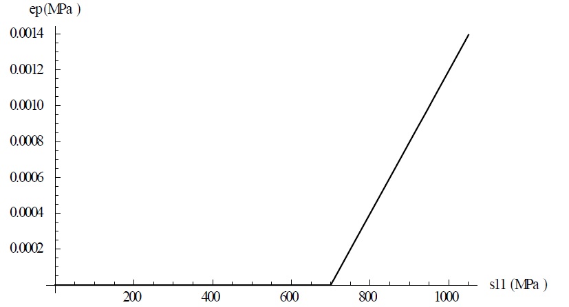
It is important to note that this condition predicts that the stresses can reach very high values before the actual failure of the material. As shown in the plot of versus given below, the value of the plastic strain parameter is only equal to 0.0014 when is equal to 1050MPa. This is because the von Mises yield criterion in this condition only predicts development of plastic strains when there is a difference between the normal stress components , , and  . However, the plane strain condition along with the condition leads to a very small increase of
  with the increase in .
View Mathematica Code
(*stress, hydrostatic stress, deviatoric stress and parameters*)
s={{s11,0,0},{0,s22,0},{0,0,s33}};
hydr=(s11+s22+s33)/3;
Sdev=FullSimplify[s-hydr*IdentityMatrix[3]];
Sdev//MatrixForm
epmax=25/100-550/200000;
hslope=N[150/epmax];
rule={Ee->200000,nu->0.3,h->hslope};
(*Relationship between stress components in the elastic regime*)
a=Solve[{0==s22/Ee-nu*s33/Ee-nu*s11/Ee,0==s33/Ee-nu*s11/Ee-nu*s22/Ee},{s22,s33}]
a=a/.rule;
Sigmavm=Sqrt[1/2*((s11-s22)^2+(s11-s33)^2+(s22-s33)^2)];
(*s11,s22 and s33 at the elastic limit*)
b=FullSimplify[Solve[{(Sigmavm/.a[[1]])==400},s11],Assumptions->{0.5>nu>0,s11>0}]
s11initial=s11/.b[[2]]
s22initial=(s22/.a[[1]])/.b[[2]]
s33initial=(s33/.a[[1]])/.b[[2]]
(*Elastic strains right before plastifying*)
ee11=FullSimplify[(s11/Ee-nu*s22/Ee-nu*s33/Ee)/.a[[1]]]/.rule
ee22=FullSimplify[(-nu*s11/Ee+s22/Ee-nu*s33/Ee)/.a[[1]]]/.rule
ee33=FullSimplify[(-nu*s11/Ee-nu*s22/Ee+s33/Ee)/.a[[1]]]/.rule
(*Manipulation of rates*)
Clear[ee22,ee11,ee33]
Sdev=Sdev/.{s11->s11[t],s22->s22[t],s33->s33[t]}
Sigmavm=Sigmavm/.{s11->s11[t],s22->s22[t],s33->s33[t]}
ee22'[t]=s22'[t]/Ee-nu*s11'[t]/Ee-nu*s33'[t]/Ee;
ee33'[t]=s33'[t]/Ee-nu*s11'[t]/Ee-nu*s33'[t]/Ee;
cep'[t]=(3/2*Sdev[[1,1]]*s11'[t]/h/Svm+3/2*Sdev[[2,2]]*s22'[t]/h/Svm+3/2*Sdev[[3,3]]*s33'[t]/h/Svm)
cep22'[t]=FullSimplify[cep'[t]*3/2*Sdev[[2,2]]/Svm]
cep33'[t]=FullSimplify[cep'[t]*3/2*Sdev[[3,3]]/Svm]
(*Solving for s22'[t] and s33'[t] in terms of s11'[t] using the zero total strain conditions*)
a=FullSimplify[Solve[{ee22'[t]+cep22'[t]==0,ee33'[t]+cep33'[t]==0},{s22'[t],s33'[t]}]]
(*Solving the ordinary differential equations for s11'[t],s22'[t] and s33'[t]*)
eq1=(((s22'[t]/.a[[1]])/.rule)/.Svm->Sigmavm)
eq2=(((s33'[t]/.a[[1]])/.rule)/.Svm->Sigmavm)
ff=NDSolve[{s22'[t]==eq1,s33'[t]==eq2,s11'[t]==1,s11[s11initial]==s11initial,s22[s11initial]==s22initial, s33[s11initial]==s33initial},{s11,s22,s33},{t,s11initial,1050}]
s22function=Piecewise[{{nu*t/(1-nu)/.rule,0<=t<=s11initial},{s22[t]/.ff[[1]],t>s11initial}}]
s33function=Piecewise[{{nu*t/(1-nu)/.rule,0<=t<=s11initial},{s33[t]/.ff[[1]],t>s11initial}}]
Plot[s22function,{t,0,1050},PlotRange->All,AxesOrigin->{0,0},AxesLabel->{"s11(MPa)","s22(MPa)"},PlotStyle->Black]
Plot[s33function,{t,0,1050},PlotRange->All,AxesOrigin->{0,0},AxesLabel->{"s11(MPa)","s33(MPa)"},PlotStyle->Black]
(*Solving the ordinary differential equations for ep'[t] and ep_ij'[t]*) cep'[t]=(cep'[t]/.Svm->Sigmavm)/.rule
eq1=ep'[t]==FullSimplify[cep'[t]]
eq2=ep11'[t]==FullSimplify[(cep'[t])*3/2*Sdev[[1,1]]/Sigmavm]
eq3=ep22'[t]==FullSimplify[(cep'[t])*3/2*Sdev[[2,2]]/Sigmavm]
eq4=ep33'[t]==FullSimplify[(cep'[t])*3/2*Sdev[[3,3]]/Sigmavm]
rule2={s11[t]->t,s22[t]->s22function,s33[t]->s33function,s22'[t]->D[s22function,t],s33'[t]->D[s33function,t],s11'[t]->1}
eq1=eq1/.rule2;eq2=eq2/.rule2;eq3=eq3/.rule2;eq4=eq4/.rule2;
a=NDSolve[{eq1,ep[s11initial]==0},ep,{t,s11initial,1050}]
b=NDSolve[{eq2,ep11[s11initial]==0},ep11,{t,s11initial,1050}]
c=NDSolve[{eq3,ep22[s11initial]==0},ep22,{t,s11initial,1050}]
d=NDSolve[{eq4,ep33[s11initial]==0},ep33,{t,s11initial,1050}]
(*Plastic strains as functions of t and their plots*)
ep11function=Piecewise[{{0,0<=t<=s11initial},{ep11[t]/.b[[1]],t>s11initial}}]
ep22function=Piecewise[{{0,0<=t<=s11initial},{ep22[t]/.c[[1]],t>s11initial}}]
ep33function=Piecewise[{{0,0<=t<=s11initial},{ep33[t]/.d[[1]],t>s11initial}}]
epfunction=Piecewise[{{0,0<=t<=s11initial},{ep[t]/.a[[1]],t>s11initial}}]
ee11function=(t/Ee-s22function/Ee*nu-s33function/Ee*nu)/.rule;
ee22function=(-nu*t/Ee+s22function/Ee-s33function/Ee*nu)/.rule;
ee33function=(-nu*t/Ee-nu*s22function/Ee+s33function/Ee)/.rule;
Plot[ep11function,{t,0,1050},PlotRange->All,AxesOrigin->{0,0},AxesLabel->{"s11(MPa)","ep11(MPa)"},PlotStyle->Black]
Plot[ep22function,{t,0,1050},PlotRange->All,AxesOrigin->{0,0},AxesLabel->{"s11(MPa)","ep22(MPa)"},PlotStyle->Black]
Plot[ep33function,{t,0,1050},PlotRange->All,AxesOrigin->{0,0},AxesLabel->{"s11(MPa)","ep33(MPa)"},PlotStyle->Black]
Plot[epfunction,{t,0,1050},PlotRange->All,AxesOrigin->{0,0},AxesLabel->{"s11(MPa)","ep(MPa)"},PlotStyle->Black]
Plot[ee11function,{t,0,1050},PlotRange->All,AxesOrigin->{0,0},AxesLabel->{"s11(MPa)","ee11(MPa)"},PlotStyle->Black]
Plot[ee22function,{t,0,1050},PlotRange->All,AxesOrigin->{0,0},AxesLabel->{"s11(MPa)","ee22(MPa)"},PlotStyle->Black]
Plot[ee33function,{t,0,1050},PlotRange->All,AxesOrigin->{0,0},AxesLabel->{"s11(MPa)","ee33(MPa)"},PlotStyle->Black]
Plot[ee11function+ep11function,{t,0,1050},PlotRange->All,AxesOrigin->{0,0},AxesLabel->{"s11(MPa)","e11(MPa)"},PlotStyle->Black]
Plot[Chop[ee22function+ep22function,10^-7],{t,0,1050},PlotRange->All,AxesOrigin->{0,0},AxesLabel->{"s11(MPa)","e22(MPa)"},PlotStyle->Black]
Plot[Chop[ee33function+ep33function],{t,0,1050},PlotRange->All,AxesOrigin->{0,0},AxesLabel->{"s11(MPa)","e33(MPa)"},PlotStyle->Black]
View Python Code
from sympy import *
import sympy as sp
import numpy as np
import matplotlib.pyplot as plt
from scipy.integrate import odeint
from scipy.interpolate import InterpolatedUnivariateSpline
sp.init_printing(use_latex = "mathjax")
s11,s22,s33,nu,E,h,Svm,t = symbols("\u03c3_{11} \u03c3_{22} \u03c3_{33} nu E h \u03c3_{vM} t")
s = Matrix([[s11,0,0],[0,s22,0],[0,0,s33]])
hydr = (s11 + s22 + s33)/3;
Sdev = simplify(s-hydr*eye(3))
display(Sdev)
epmax = 25/100-550/200000
hslope = 150/epmax
display(epmax)
display(hslope)
rule = {E:200000, nu:0.3, h:hslope}
display("Relationship between stress components in the elastic regime")
a = solve((s22/E-nu*s33/E-nu*s11/E,s33/E-nu*s11/E-nu*s22/E),s22,s33)
for key in a:
    a[key] = a[key].subs(rule)
display(a)
Sigmavm = sqrt(1/2*((s11-s22)**2+(s11-s33)**2+(s22-s33)**2))
Sigmavmsub = simplify(Sigmavm.subs(a))
display("s11, s22 and s33 at the elastic limit")
b = solve((Sigmavmsub-400),sqrt(s11**2), dict = true)
display(b[0])
display("Since s_11>0:")
b = {s11:700}
display(b)
s11initial = s11.subs(b)
s22initial = (s22.subs(a)).subs(b)
s33initial = (s33.subs(a)).subs(b)
display(s11initial,s22initial,s33initial)
display("Elastic strains right before plastifying")
ee11 = simplify((s11/E-nu*s22/E-nu*s33/E).subs(a)).subs(rule)
ee22 = simplify((-nu*s11/E+s22/E-nu*s33/E).subs(a)).subs(rule)
ee33 = simplify((-nu*s11/E-nu*s22/E+s33/E).subs(a)).subs(rule)
display(ee11,ee22,ee33)
display("Manipulation of rates")
s11t,s22t,s33t = Function('\u03c3_{11}')(t),Function('\u03c3_{22}')(t),Function('\u03c3_{33}')(t)
Sdev = Sdev.subs({s11:s11t,s22:s22t,s33:s33t})
Sigmavm = Sigmavm.subs({s11:s11t,s22:s22t,s33:s33t})
display(Sdev,Sigmavm)
ee22p = s22t.diff(t)/E-nu*s11t.diff(t)/E-nu*s33t.diff(t)/E
ee33p = s33t.diff(t)/E-nu*s11t.diff(t)/E-nu*s33t.diff(t)/E
cepp = 3/2*Sdev[0,0]*s11t.diff(t)/h/Svm+3/2*Sdev[1,1]*s22t.diff(t)/h/Svm+3/2*Sdev[2,2]*s33t.diff(t)/h/Svm
cep22p = simplify(cepp*3/2*Sdev[1,1]/Svm)
cep33p = simplify(cepp*3/2*Sdev[2,2]/Svm)
display(cepp,cep22p,cep33p)
display("Solving for s22'[t] and s33'[t] in terms of s11'[t] using the zero total strain conditions")
a = solve((ee22p+cep22p,ee33p+cep33p),s22t.diff(t),s33t.diff(t))
display(a)
display("Solving the ordinary differential equations for s11'[t],s22'[t] and s33'[t]")
eq1 = ((s22t.diff(t).subs(a)).subs(rule)).subs(Svm,Sigmavm)
eq2 = ((s33t.diff(t).subs(a)).subs(rule)).subs(Svm,Sigmavm)
equ1 = eq1.subs({s11t:s11,s22t:s22,s33t:s22,s11t.diff(t):1})
display(eq1,eq2)
equ2 = eq2.subs({s11t:s11,s22t:s33,s33t:s33,s11t.diff(t):1})
def rhs1(y,t):
    f = sp.lambdify([s11,s22],equ1)
    f = f(y[0],y[1])
    return [1,f]
def rhs2(y,t):
    f = sp.lambdify([s11,s33],equ2)
    f = f(y[0],y[1])
    return [1,f]
s11initial = float(s11initial)
t1 = np.linspace(s11initial,1050,20)
yzero1 = [s11initial,s22initial]
yzero2 = [s11initial,s33initial]
ff1 = odeint(rhs1,yzero1,t1)
ff2 = odeint(rhs2,yzero2,t1)
display("Solving the ordinary differential equations for ep'[t] and ep_ij'[t]")
cepp = (cepp.subs(rule)).subs(Svm,Sigmavm)
display(cepp)
eq1 = simplify(cepp)
eq2 = simplify(cepp*3/2*Sdev[0,0]/Sigmavm)
eq3 = simplify(cepp*3/2*Sdev[1,1]/Sigmavm)
eq4 = simplify(cepp*3/2*Sdev[2,2]/Sigmavm)
display(eq1,eq2,eq3,eq4)
rule2 = {s11t:s11,s22t:s22,s33t:s33,s11t.diff(t):1}
def integralsolve(eq, ff1,ff2):
    eptp = simplify((((eq.subs(a)).subs(Svm,Sigmavm)).subs(rule)).subs(rule2))
    f = sp.lambdify([s11,s22,s33],eptp)
    sol = f(ff1[:,0],ff1[:,1],ff2[:,1])
    f2 = InterpolatedUnivariateSpline(ff1[:,0],sol,k=1)
    return [f2.integral(s11initial,ff1[i,0]) for i in range(20)]
epfunction = integralsolve(eq1,ff1,ff2)
ep11function = integralsolve(eq2,ff1,ff2)
ep22function = integralsolve(eq3,ff1,ff2)
ep33function = integralsolve(eq4,ff1,ff2)
#eeFunctions
ee11function = sp.lambdify([s11,s22,s33],(s11/E-s22/E*nu-s33/E*nu).subs(rule))
sol_ee11 = ee11function(ff1[:,0],ff1[:,1],ff2[:,1])
ee22function = sp.lambdify([s11,s22,s33],(-nu*s11/E+s22/E-s33/E*nu).subs(rule))
sol_ee22 = ee22function(ff1[:,0],ff1[:,1],ff2[:,1])
ee33function = sp.lambdify([s11,s22,s33],(-nu*s11/E-nu*s22/E+s33/E).subs(rule))
sol_ee33 = ee33function(ff1[:,0],ff1[:,1],ff2[:,1])
lambda1 = lambdify(t,(t*nu/(1-nu)).subs(rule))
lambda2 = lambdify(t,(t/E-nu*t/(1-nu)/E*nu-nu*t/(1-nu)/E*nu).subs(rule))
xL = np.linspace(0,s11initial,2)
fig,ax = plt.subplots(6,2, figsize = (20,30))
plt.setp(ax[0,0], xlabel = "s11",ylabel="s22")
ax[0,0].plot(ff1[:,0],ff1[:,1],'b-')
ax[0,0].plot(xL,lambda1(xL),'b-')
plt.setp(ax[0,1], xlabel = "s11",ylabel="s33")
ax[0,1].plot(ff2[:,0],ff2[:,1],'b-')
ax[0,1].plot(xL,lambda1(xL),'b-')
plt.setp(ax[1,0], xlabel = "s11",ylabel="ep")
ax[1,0].plot(ff1[:,0],epfunction,'b-')
ax[1,0].plot(xL,[0,0], 'b-')
plt.setp(ax[1,1], xlabel = "s11",ylabel="ep11")
ax[1,1].plot(ff1[:,0],ep11function,'b-')
ax[1,1].plot(xL,[0,0], 'b-')
plt.setp(ax[2,0], xlabel = "s11",ylabel="ep22")
ax[2,0].plot(ff1[:,0],ep22function,'b-')
ax[2,0].plot(xL,[0,0], 'b-')
plt.setp(ax[2,1], xlabel = "s11",ylabel="ep33")
ax[2,1].plot(ff1[:,0],ep33function,'b-')
ax[2,1].plot(xL,[0,0], 'b-')
plt.setp(ax[3,0], xlabel = "s11",ylabel="ee11")
ax[3,0].plot(ff1[:,0],sol_ee11,'b-')
ax[3,0].plot(xL,lambda2(xL),'b-')
plt.setp(ax[3,1], xlabel = "s11",ylabel="ee22")
ax[3,1].plot(ff1[:,0],sol_ee22,'b-')
ax[3,1].plot(xL,[0,0],'b-')
plt.setp(ax[4,0], xlabel = "s11",ylabel="ee33")
ax[4,0].plot(ff1[:,0],sol_ee33,'b-')
ax[4,0].plot(xL,[0,0],'b-')
plt.setp(ax[4,1], xlabel = "s11",ylabel="e11")
ax[4,1].plot(ff1[:,0],sol_ee11+ep11function,'b-')
ax[4,1].plot(xL,lambda2(xL),'b-')
plt.setp(ax[5,0], xlabel = "s11",ylabel="e22")
ax[5,0].plot(ff1[:,0],sol_ee22+ep22function,'b-')
ax[5,0].plot(xL,[0,0],'b-')
ax[5,0].set_ylim([-1,1])
plt.setp(ax[5,1], xlabel = "s11",ylabel="e33")
ax[5,1].plot(ff1[:,0],sol_ee33+ep33function,'b-')
ax[5,1].plot(xL,[0,0],'b-')
ax[5,1].set_ylim([-1,1])
for i in range(6):
    for j in range(2):
        ax[i,j].grid(True,which='both')
        ax[i,j].axvline(x=0,color='k',alpha=0.5)
        ax[i,j].axhline(y=0,color = 'k',alpha=0.5)
plt.show()
Example 2: Nonlinear Kinematic Hardening
The “true” stress versus “true strain” of a metal that follows the nonlinear kinematic hardening model with a constant size of the yield surface is given in the following table.
| True Strain (%) | 0 | 0.09 | 0.18 | 2.045 | 4.905 | 9.495 | 18.235 | 23.975 |
| Stress(MPa) | 0 | 180 | 360 | 395 | 450 | 510 | 570 | 590 |
Assume that  GPa and
  . Find the values of
  and
and  such that the Armstrong-Frederick evolution law for the backstress can be used to describe the metal’s behaviour. Then, find the different nonzero elastic and plastic strain components and the components of the backstress tensor associated with the following loading steps:
Step 1: A specimen of this material is incrementally loaded in shear such that
 MPa.
MPa.Step 2: The stress
 is removed
Step 3:
is increased to 500 MPa.
Solution
The true plastic strain versus true stress can be computed by subtracting the elastic strain component and thus, the relationship between and is according to the following table:
| 0 | 0 | 0 | 0.0185 | 0.0468 | 0.0924 | 0.1795 | 0.2368 |
| Stress(MPa) | 0 | 180 | 360 | 395 | 450 | 510 | 570 | 590 |
The material starts to yield when  MPa and since the material is assumed to have a constant size for the yield surface, then
  MPa. Integration of the Armstrong-Frederick material model yields the following relationship for uniaxial loading:
![\[\alpha_{11} = \frac{C}{\gamma} (1 - e^{-\gamma \overline{\varepsilon^p}})\]](https://engcourses-uofa.ca/wp-content/ql-cache/quicklatex.com-b63ee97b620b430aec8493ae5c1fe439_l3.png "Rendered by QuickLaTeX.com")
Where  . The values of and that would produce the best fit between the given data and the model can be found to be equal to 2352.3 and 8.97417 respectively using Mathematica.
View Mathematica Code
ss={{0,0},{0.0185,395-360},{0.0468,450-360},{0.0924,510-360},{0.1795,570-360},{0.2368,590-360}};
a=FindFit[ss,Cc/gamma*(1-Exp[-gamma*ep]),{Cc,gamma},ep]
Cc=Cc/.a[[1]]
gamma=gamma/.a[[2]]
ss2=Table[{ss[[i,1]],Cc/gamma*(1-Exp[-gamma*ss[[i,1]]])},{i,1,6}];
ListPlot[{ss,ss2},Joined->True,AxesOrigin->{0,0}]
View Python Code
import matplotlib.pyplot as plt
from scipy.optimize import curve_fit
import numpy as np
def func(x,a,b):
    return a/b*(1-np.exp(-b*x))
xdata = np.array([0,0.0185,0.0468,0.0924,0.1795,0.2368])
ydata = np.array([0,35,90,150,210,230])
popt,pcov = curve_fit(func,xdata,ydata)
display("a value =",popt[0],"b value =",popt[1])
xfundata = np.array([i/20*0.25 for i in range(20)])
yfundata = func(xfundata,*popt)
plt.plot(xdata,ydata,'o',label='Data')
plt.plot(xfundata,yfundata,'r-',label='Best Fit: a=%5.1f, b=%5.5f'%tuple(popt))
plt.xlabel('x')
plt.ylabel('y')
plt.legend()
Step 1
At the beginning of the analysis, the values of the components  are equal to zero. As the material is first loaded in shear, the first initial yield is obtained when
  MPa, therefore:
![\[\sqrt{3\sigma_{12}^2} = 360 MPa \Rightarrow \sigma_{12} = 207.85 MPa\]](https://engcourses-uofa.ca/wp-content/ql-cache/quicklatex.com-687c9a24af26c9c0b673c78081adb40e_l3.png "Rendered by QuickLaTeX.com")
At this instant, the only nonzero elastic strain components are  . Beyond the elastic limit, an increment
  is accompanied by plastic strains and a transition of the yield surface according to the evolution of the backstress. The consistency condition can be used to find the value of :
![\[\Delta f = 0 = \sum_{i,j=1}^3 \frac{\partial f}{\partial \sigma_{ij}} \Delta \sigma_{ij} + \sum_{i,j=1}^3 \frac{\partial f}{\partial \alpha_{ij}} \Delta \alpha_{ij} - \frac{d\sigma_{Y \alpha}}{d\overline{\varepsilon^p}} \Delta \overline{\varepsilon^p} = 0\]](https://engcourses-uofa.ca/wp-content/ql-cache/quicklatex.com-5ac4ea87faa3ef5aa243322dac6bf3dc_l3.png "Rendered by QuickLaTeX.com")
Since the size of the yield surface is given in this problem as a constant, then the value of  is equal to 0. The only nonzero stress increment components in the above equations are
  and
and  . Utilizing the Armstrong-Frederick evolution law to substitute for the components
  results in the following expression:
![\[\frac{\partial f}{\partial \sigma_{12}} \Delta \sigma_{12} + \frac{\partial f}{\partial \sigma_{21}}\Delta \sigma_{21} + \sum_{i,j=1}^3 \Big(\frac{\partial f}{\partial \alpha_{ij}} \Big(\frac{C(\sigma_{ij} - \alpha_{ij})}{\sigma_{Y \alpha}} - \gamma \alpha_{ij}\Big)\Big) \Delta \overline{\varepsilon^p} = 0\]](https://engcourses-uofa.ca/wp-content/ql-cache/quicklatex.com-af895145d13006c03367b0e32517125a_l3.png "Rendered by QuickLaTeX.com")
The only nonzero components of the stress and the backstress tensor components would be ,  ,
,  , and
, and  . Therefore:
![\[\frac{\partial f}{\partial \sigma_{12}} \Delta \sigma_{12} + \frac{\partial f}{\partial \sigma_{21}} \Delta \sigma_{21} + \Big(\frac{\partial f}{\partial \alpha_{21}}\Big(\frac{C(\sigma_{12} - \alpha_{12})}{\sigma_{Y \alpha}} - \gamma \alpha_{12}\Big) + \frac{\partial f}{\partial \alpha_{21}} \Big(\frac{C(\sigma_{21} - \alpha_{21})}{\sigma_{Y \alpha}} - \gamma \alpha_{21} \Big) \Big) \Delta \overline{\varepsilon^p} = 0\]](https://engcourses-uofa.ca/wp-content/ql-cache/quicklatex.com-5d1a88772a068e481a446749b1865ece_l3.png "Rendered by QuickLaTeX.com")
The above relationship can be integrated numerically to find the value of as increases from the initial yield at  MPa up to MPa. The following table shows the numerical integration process with an increment
  MPa.
MPa.
 | |  | | |  |
| 207.85 | 0 | 0.866 | 20 | 0.0147 | 20 |
| 227.85 | 20 | 0.866 | 20 | 0.0170 | 20 |
| 247.85 | 40 | 0.866 | 20 | 0.020 | 20 |
| 267.85 | 60 | 0.866 | 20 | 0.0244 | 20 |
| 287.85 | 80 | 0.866 | 12.15 | 0.0190 | 12.15 |
| 300 | 92.15 |
The value of the plastic strain parameter at the end of the loading process is the sum of the individual increments:
![\[\overline{\varepsilon^p} = 0.0951\]](https://engcourses-uofa.ca/wp-content/ql-cache/quicklatex.com-e9f39f131df1ebc11f01df75348d8a68_l3.png "Rendered by QuickLaTeX.com")
Also, the value of the non-zero backstress tensor components  is equal to the sum of the individual increments:
![\[\alpha_{12} = \alpha_{21} = 92.15 MPa\]](https://engcourses-uofa.ca/wp-content/ql-cache/quicklatex.com-e02bc08b83eebf06f169774a69a2daee_l3.png "Rendered by QuickLaTeX.com")
The nonzero elastic strain components are:
![\[\varepsilon_{12}^e = \varepsilon_{21}^e = \frac{300}{2G} = 0.00195\]](https://engcourses-uofa.ca/wp-content/ql-cache/quicklatex.com-545fbb31d0979b8a434462ffae7f36c7_l3.png "Rendered by QuickLaTeX.com")
The nonzero plastic strain components can be calculated by numerical integration of the following formula:
![\[\Delta \varepsilon_{12}^p = \Delta \varepsilon_{21}^p = \Delta \overline{\varepsilon^p} \frac{\partial f}{\partial \sigma_{12}}\]](https://engcourses-uofa.ca/wp-content/ql-cache/quicklatex.com-644859739c344e040adeec1442b34af8_l3.png "Rendered by QuickLaTeX.com")
The following table shows the values of the plastic strain components at the end of this load step:
 | |  |  |  | 0.866 | 0.0147 | 0.0128 | 207.85 | 0 |
| 0.866 | 0.0170 | 0.0147 | 227.85 | 0.0128 |
| 0.866 | 0.0200 | 0.0173 | 247.85 | 0.0274 |
| 0.866 | 0.0244 | 0.0211 | 267.85 | 0.0448 |
| 0.866 | 0.0190 | 0.0164 | 287.85 | 0.0659 |
| 300 | 0.0824 |
Step 2
The unloading in step 2 occurs in the elastic regime since as is reduced to zero, the yield function is negative:
![\[\sigma_{vM}|_{\sigma - \alpha} = \sqrt{3(\sigma_{12} - 92.15)(\sigma_{12}-92.15)} = \sqrt{3} (\sigma_{12} - 92.15) < \sigma_{Y\alpha} = 360\]](https://engcourses-uofa.ca/wp-content/ql-cache/quicklatex.com-e1213a4599f4551a3ba0056b52856d38_l3.png "Rendered by QuickLaTeX.com")
At the end of step 2, the elastic strains are zero while no change occurs in the plastic strain components, the plastic strain parameter nor in the components of the backstress tensor:
![\[\varepsilon_{12}^p = \varepsilon_{21}^p = 0.0824 \hspace{5mm} \alpha_{12} = \alpha_{21} = 92.15 MPa \hspace{5mm} \overline{\varepsilon^p} = 0.0951\]](https://engcourses-uofa.ca/wp-content/ql-cache/quicklatex.com-13b4f1f540c03089468f177abb615ce4_l3.png "Rendered by QuickLaTeX.com")
Step 3
Loading in step 3 will occur elastically until the yield function reaches the value of zero. In this instance, the value of can be obtained by solving the following equation:
![\[\sigma_{vM}|_{\sigma - \alpha} = \sqrt{3(-92.15)^2 + \frac{3}{2} \Big(\frac{2}{3} \sigma_{11} \Big)^2 + 3\Big(\frac{-1}{3} \sigma_{11} \Big)^2} = 360 \Rightarrow \sigma_{11} = 322.684 MPa\]](https://engcourses-uofa.ca/wp-content/ql-cache/quicklatex.com-a46905d3571f893b030c256ed462a9da_l3.png "Rendered by QuickLaTeX.com")
As increases beyond this limit, plastic strain develops and the consistency condition can be used to find the increment in the plastic strain parameter as follows:
![\[\Delta f = 0 = \sum_{i,j=1}^3 \frac{\partial f}{\partial \sigma_{ij}} \Delta \sigma_{ij} + \sum_{i,j=1}^e \frac{\partial f}{\partial \alpha_{ij}} \Delta \alpha_{ij} - \frac{d\sigma_{Y \alpha}}{d \overline{\varepsilon^p}} \Delta \overline{\varepsilon^p} = 0\]](https://engcourses-uofa.ca/wp-content/ql-cache/quicklatex.com-a037a5158bdab4810e8eabd1f9b97efa_l3.png "Rendered by QuickLaTeX.com")
In the above equation,  and the only nonzero stress increment component is
  . Utilizing the Armstrong-Frederick evolution law to substitute for the components
  results in the following expression:
![\[\frac{\partial f}{\partial \sigma_{11}} \Delta \sigma_{11} + \sum_{i,j=1}^3 \Big(\frac{\partial f}{\partial \alpha_{ij}} \Big(\frac{C(\sigma_{ij} - \alpha_{ij})}{\sigma_{Y \alpha}} - \gamma \alpha_{ij} \Big) \Big) \Delta \overline{\varepsilon^p} = 0\]](https://engcourses-uofa.ca/wp-content/ql-cache/quicklatex.com-7f1fb60ca434084a4bbb37f4ded9211b_l3.png "Rendered by QuickLaTeX.com")
The only nonzero components of the stress and the backstress tensor components would be ,  , , and . Therefore:
![\[\frac{\partial f}{\partial \sigma_{11}} \Delta \sigma_{11} + \Big(\frac{\partial f}{\partial \alpha_{11}} \Big(\frac{C(\sigma_{11} - \alpha_{11})}{\sigma_{Y \alpha}} -\gamma \alpha_{11}\Big) + \frac{\partial f}{\partial \alpha_{12}} \Big(\frac{C(\sigma_{12} -\alpha_{12})}{\sigma_{Y \alpha}} - \gamma \alpha_{12} \Big)\]](https://engcourses-uofa.ca/wp-content/ql-cache/quicklatex.com-8191a99a426641fbed4dc3e4367e8319_l3.png "Rendered by QuickLaTeX.com")
![\[+ \frac{\partial f}{\partial \alpha_{21}} \Big(\frac{C(\sigma_{21}-\alpha_{21})}{\sigma_{Y \alpha}} - \gamma \alpha_{21} \Big)\Big) \Delta \overline{\varepsilon^p} = 0\]](https://engcourses-uofa.ca/wp-content/ql-cache/quicklatex.com-5078def5cf3907ab0fc961e0b7d42e3c_l3.png "Rendered by QuickLaTeX.com")
The above relationship can be integrated numerically to find the value of as increases from the initial yield at  MPa up to
  MPa. The following table shows the numerical integration process with an increment \Delta
  MPa.
MPa.
| MPa | | (MPa) | (MPa) |  |  | |  (MPa) (MPa) |  (MPa) (MPa) |
| 322.68 | 0 | 92.15 | 20 | 0.8963 | 0.3840 | 0.0060 | 12.65 | -8.58 |
| 342.68 | 12.65 | 83.58 | 20 | 0.9168 | 0.3482 | 0.0067 | 13.50 | -8.56 |
| 362.68 | 26.15 | 75.02 | 20 | 0.9348 | 0.3216 | 0.0073 | 14.33 | -8.48 |
| 382.68 | 40.47 | 66.53 | 20 | 0.950.6 | 0.2772 | 0.0081 | 15.14 | -8.34 |
| 402.68 | 55.61 | 58.19 | 20 | 0.9641 | 0.2425 | 0.0090 | 15.92 | -8.12 |
| 422.68 | 71.53 | 50.07 | 20 | 0.9754 | 0.2086 | 0.0101 | 16.65 | -7.82 |
| 442.68 | 88.18 | 42.25 | 20 | 0.9847 | 0.1760 | 0.0114 | 17.34 | -7.45 |
| 462.68 | 105.52 | 34.80 | 20 | 0.9921 | 0.1450 | 0.0129 | 17.96 | -6.99 |
| 482.68 | 123.47 | 27.81 | 17.316 | 0.9978 | 0.1159 | 0.0129 | 16.02 | -5.58 |
| 500.00 | 139.49 | 22.23 |
The increments in the plastic strain components can be computed as follows:
![\[\Delta \varepsilon_{12}^p = \Delta \varepsilon_{21}^p = \Delta \overline{\varepsilon^p} \frac{\partial f}{\partial \sigma_{12}} = -\Delta \overline{\varepsilon^p} \frac{\partial f}{\partial \alpha_{12}} \hspace{5mm} \Delta \varepsilon_{11}^p = \Delta \overline{\varepsilon^p} \frac{\partial f}{\partial \sigma_{11}}\]](https://engcourses-uofa.ca/wp-content/ql-cache/quicklatex.com-ad9afe6cf76fdd1ab5ddf610bad60c5a_l3.png "Rendered by QuickLaTeX.com")
The following table shows the calculations of the increments in the plastic strain components:
| (MPa) |  |  (MPa) (MPa) | (MPa) | | |  | |
| 0.0060 | -0.0023 | 0.0054 | 322.68 | 0.0951 | 0 | 0 | 0.0824 |
| 0.0067 | -0.0023 | 0.0061 | 342.68 | 0.1011 | 0.0054 | -0.0027 | 0.0801 |
| 0.0073 | -0.0023 | 0.0068 | 362.68 | 0.1077 | 0.0114 | -0.0057 | 0.0778 |
| 0.0081 | -0.0022 | 0.0077 | 382.68 | 0.1150 | 0.0183 | -0.0091 | 0.0755 |
| 0.0090 | -0.0022 | 0.0087 | 402.68 | 0.1231 | 0.0259 | -0.0130 | 0.0733 |
| 0.0101 | -0.0021 | 0.0098 | 422.68 | 0.1321 | 0.0346 | -0.0173 | 0.0711 |
| 0.0114 | -0.0020 | 0.0112 | 442.68 | 0.1422 | 0.0444 | -0.0222 | 0.0690 |
| 0.0129 | -0.0019 | 0.0128 | 462.68 | 0.1535 | 0.0556 | -0.0278 | 0.0670 |
| 0.0129 | -0.0015 | 0.0129 | 482.68 | 0.1665 | 0.0685 | -0.0342 | 0.0651 |
| 500.00 | 0.1794 | 0.0814 | -0.0407 | 0.0636 |
Thus, at the end of step 3, the following are the values of the non-zero backstress components, elastic strain components, and plastic strain components:
![\[\sigma_{11} = 139.49 \hspace{5mm} \alpha_{12} = \alpha_{21} = 22.23 \hspace{5mm} \varepsilon_{11}^e = \frac{500}{E} = 0.0025 \hspace{5mm} \varepsilon_{22}^e = \varepsilon_{33}^e = -0.00075\]](https://engcourses-uofa.ca/wp-content/ql-cache/quicklatex.com-1a75c3b43e71d8bfbf4cee43b75db2ca_l3.png "Rendered by QuickLaTeX.com")
![\[\varepsilon_{11}^p = 0.0814 \hspace{5mm} \varepsilon_{22}^p = \varepsilon_{33}^p = -0.0407 \hspace{5mm} \varepsilon_{12}^e = \varepsilon_{21}^p = 0.0636\]](https://engcourses-uofa.ca/wp-content/ql-cache/quicklatex.com-2e8790b618aaf36724ef52251309b5ff_l3.png "Rendered by QuickLaTeX.com")
This example shows the behaviour of the kinematic hardening model under multiple load steps. The application of a shear stress in an initial load step developed plastic shear strains and a backstress components  . When the shear stress was removed and a uniaxial stress was applied, the material started to yield at a stress value of
  MPa. In addition, contrary to the isotropic hardening model, this model predicts a decrease in the plastic shear strain components with the increase in .
Problems
The engineering strain-engineering stress curve for a steel material follows the numbers in the table shown. Assuming that
 MPa and Poisson’s ratio .
Strain (%) 0 0.085 0.17 2.06 5.02 9.95 20 27.07 Stress(MPa) 0 178.4 356.4 382 428.5 463.8 472.5 456.2 Plot the true strain – true stress curve.
Plot the relationship between the stress and the true plastic strain.
Find the yield stress given the two criteria: 0.2% offset and the 0.5% strain.
Find a Ramberg-Osgood approximation
 ,
, for the relationship between and by minimizing the square root of the error in the observations compared to the model. Hints:
You can use one of the Mathematica functions NMinimize, Fit or FindFit to find
, such that the experimental values would have the best fit to the equation 
The Ramberg-Osgood approximation assumes that the point
 belongs to the curve of the yield stress vs. plastic strain parameter. When curve fitting, you shouldn’t use a point with a yield stress corresponding to zero plastic strain.
Use the incremental Von-Mises isotropic hardening theory to find the elastic strains and the plastic strain parameter
for the following three plane stress states. Assume that the stresses increase linearly together starting from zero (i.e., no unloading).State 1:
 MPa,
MPa,  MPa,
MPa,  MPa
MPaState 2:
 MPa,
MPa,  MPa,
MPa,  MPa
MPaState 3:
 MPa,
MPa,  MPa,
MPa,  MPa
MPa
Describe three different history paths that lead to the stress state
 MPa and
In a three dimensional state of stress, during plastic deformation the increment in the plastic strain energy that is dissipated (irrecoverable plastic strain) in the material per unit volume is equal to
 . Show that when the associated flow rule of von-Mises plasticity is used to calculate the plastic strain components, then the increment in the plastic strain energy is equal to
  , i.e., the product of the equivalent stress and the increment in the equivalent plastic strain.
Let
 be the von Mises yield function, where, \sigma_{vM} is the von Mises stress and is the uniaxial yield stress. If
  are the Cauchy and the deviatoric stress tensors respectively, show the following equality:
If the stress-strain relationship of a material in simple tension is given by:

Where
 ,
,  , and
, and  are material constants.Using the incremental Von-Mises theory, show the following expression for the case of pure shear:
Where
 is the applied shear stress, and
  is the total shear strain. This example is from the book “Plasticity for Structural Engineers” by Wai-Fah Chen.
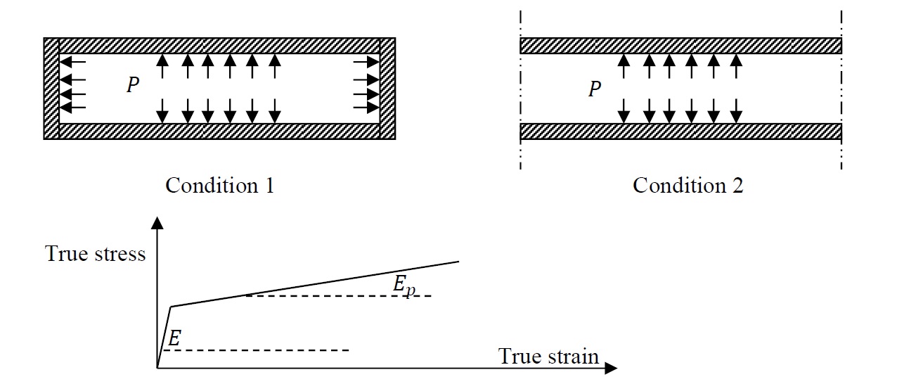
A pipe with capped ends (condition 1 in the figure below) and another infinitely long pipe (condition 2 in the figure below) are subjected to an internal pressure
 . The two pipes are made out of a steel material with Young’s modulus and Poisson’s ratio
  . The true stress versus true strain relationship obtained from a uniaxial test follows a bilinear relationship with the initial slope equal to and the strain hardening slope equal to
  . The slope of the true stress versus plastic strain relationship is designated . If the yield stress at the end of the initial elastic portion of the curve is equal to then:
For EACH pipe, find the pressure
 (the pressure at the onset of yield) in terms of the material parameters given.
Find the relationship between
, , and .Assuming that the pressure inside the pipes increases to
 , find the associated three dimensional plastic strain increments in EACH of the two cases.
A long steel thin-walled tube with diameter
 and wall thickness is subjected to an interior pressure
  and an external pressure
  . The ends of the tube are closed. The external pressure is assumed not to affect the axial stress component of the tube. Assuming that the material obeys the Von-Mises isotropic hardening theory and using the following relationship between the plastic strain parameter and the yield stress obtained from uniaxial experiments (
 is a material parameter):
Assuming that the axial direction is the direction of the basis vector
and the circumferential direction is the direction of the basis vector  show that the plastic strain components and developed through the following load paths are:


Where
 Also, sketch the yield surfaces and the loading paths in the
  space and explain the results obtained. Hint:
  ,
,  ,
,  .
This example is from the book “Plasticity for Structural Engineers” by Wai-Fah Chen
.
This example is from the book “Plasticity for Structural Engineers” by Wai-Fah ChenIn a confined compression test a compressive
is applied while keeping , and equal to zero. If a metal specimen that follows the von Mises yield criterion and the associated flow rule is subjected to a confined compression test, as is increased, will the metal ever deform plastically or not. Justify your answer.A cylindrical metal piece is subjected to a lateral stress of -75MPa and a tensile vertical stress of 300MPa. Assume that the magnitudes of the stresses increase linearly together. If the yield stress is 200MPa and the relationship between the von Mises stress in MPa and the equivalent plastic strain
is linear with a slope of 10000:Calculate the stresses at the onset of yielding.
Find the total strains at the onset of yielding.
Find the total strains when the stresses reach the maximum value.
A piece of metal obeys the nonlinear kinematic hardening model with a constant size of the yield surface and the Armstrong-Frederick evolution law for the backstress. The following is the engineering stress-strain curve obtained when the material is stretched in a uniaxial stress state.
Strain (%) 0 0.085 0.17 2.06 5.02 9.95 20 27.07 Stress(MPa) 0 178.4 356.4 382 428.5 463.8 472.5 456.2 If a specimen of this material is subjected to the following load steps:
Step 1, a uniaxial stress component
such that  .
.Step 2, the stress is removed.
Step 3, a uniaxial stress component
.
Find the true stress
versus the “apparent” plastic strain component relationship obtained in step 3 using the nonlinear kinematic hardening model of the incremental plasticity with a constant size of the yield surface.The true stress true strain relationship of a metal in simple tension is given by:

which is an elastic-linear hardening plastic stress strain relationship with
 being the initial yield stress. The material follows the von Mises isotropic hardening plasticity model. Find the total strains in the following two different paths:
- increases from 0 to and then remains constant. When reaches , increases from 0 to

- and increase linearly together from to (
 )
)
Show that the stress-strain relationship of a metal that follows the Armstrong-Frederick plasticity material model with a constant size of the yield surface is given by:

Where
and are the Armstrong-Frederick material constants and is the initial yield stress.A metal follows the combined nonlinear kinematic-isotropic hardening plasticity model such that the kinematic hardening model follows the Armstrong-Frederick evolution law with
 and
and  while the isotropic hardening model follows the relationship
in units of MPa with
 and
and  .
.Show that the relationship between the applied uniaxial stress
and is given by:
Note that the above relationship between
and implies that the value of the initial yield stress  MPa.
MPa.Find the total strains and the components of the backstress tensor at the end of the following path:
increases from 0 to 200MPa and then remains constant. When reaches 200MPa, increases from 0 to 150MPa.