
Calculus: Vector Calculus in Cylindrical Coordinate Systems
Introduction
Polar Coordinate System
Consider the representation of a geometric plane using  with a chosen but arbitrary origin. The directions at every point in the plane are defined using the basis vectors
  and
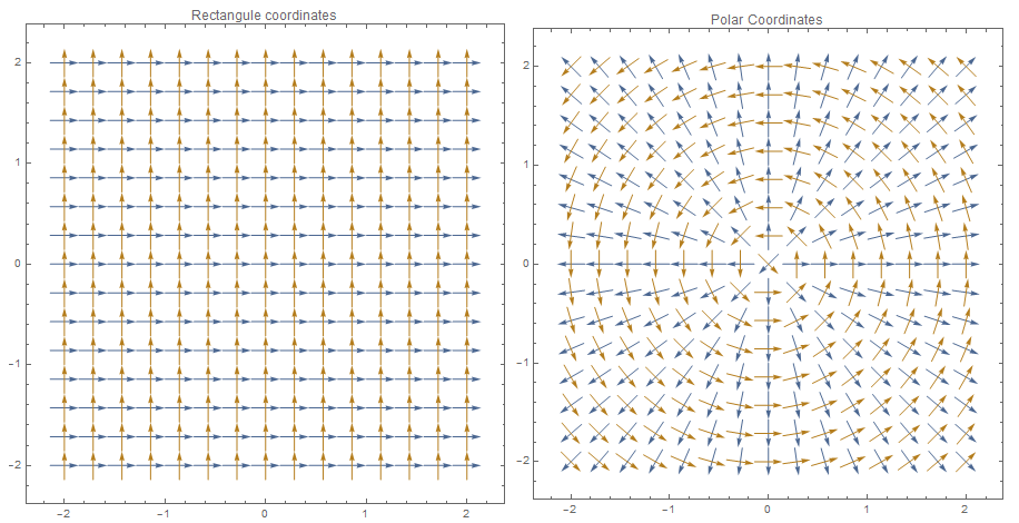
and  (Fig 1 left). In certain situations, it is more convenient to define directions or basis vectors at every point such that the first direction (first basis vector) points away from the origin (blue arrows in Fig 1 right) and the second direction is perpendicular to the first direction while maintaining the right hand rule (yellow arrows in Fig 1 right). Given that the coordinates of a point in the geometric plane are given by
  and
and  , then, we can define at every point the following relations:
![\[\begin{split} x_1&=r\cos\theta\\ x_2&=r\sin\theta \end{split} \]](https://engcourses-uofa.ca/wp-content/ql-cache/quicklatex.com-103f0048da7b1f4901daa0cc8864ddfd_l3.png "Rendered by QuickLaTeX.com")
with the inverse relationship:
![\[\begin{split} r&=\sqrt{x_1^2+x_2^2}\\ \theta&=\arctan[x_1,x_2] \end{split}\]](https://engcourses-uofa.ca/wp-content/ql-cache/quicklatex.com-c71a2e577a8596968b28e635d23e9579_l3.png "Rendered by QuickLaTeX.com")
taking into consideration the quadrant of and . It is important to note that the function ![\arctan[x1,x2]](https://engcourses-uofa.ca/wp-content/ql-cache/quicklatex.com-6607fd2e7532e89e99d5939cb3767327_l3.png "Rendered by QuickLaTeX.com") is not defined at the origin. It is also important to note that
is not defined at the origin. It is also important to note that  and
and  are themselves vector fields. represents a vector field of unit vectors that are pointing away from the origin and represents a vector field of unit vectors perpendicular to the vectors of the vector field maintaining the right hand orientation (Fig 1 left). Using a simple change of coordinates, the new basis set
  at a point represented by the coordinates and (or the corresponding r and \theta) can be related to the Cartesian basis
  and
and  using the relationships:
![\[\begin{split} e_r&=\cos(\theta)e_1+\sin(\theta)e_2\\ e_\theta&=-\sin(\theta)e_1+\cos(\theta)e_2 \end{split} \]](https://engcourses-uofa.ca/wp-content/ql-cache/quicklatex.com-402500631f5a4b88018bd34213942036_l3.png "Rendered by QuickLaTeX.com")
Therefore, the coordinate transformation from the Cartesian basis to the polar coordinate system is described at every point using the matrix  :
:
![\[ Q=\left(\begin{matrix}\cos(\theta)&\sin(\theta)\\-\sin(\theta)&\cos(\theta)\end{matrix}\right) \]](https://engcourses-uofa.ca/wp-content/ql-cache/quicklatex.com-dfc035baeac373ee9f38cc302da8f862_l3.png "Rendered by QuickLaTeX.com")
As the vector fields and are functions of the two real numbers  , and
, and  , then, we can find the derivatives of and as follows:
![\[ e_r=\cos(\theta) e_1+\sin (\theta) e_2\Rightarrow \begin{cases}\frac{\partial e_r}{\partial r}=0\\ \frac{\partial e_r}{\partial \theta}=-\sin(\theta)e_1+\cos(\theta)e_2=e_\theta\end{cases} \]](https://engcourses-uofa.ca/wp-content/ql-cache/quicklatex.com-f9bb4a2b05b522f0cd99910ffb970889_l3.png "Rendered by QuickLaTeX.com")
![\[ e_\theta=-\sin(\theta) e_1+\cos (\theta) e_2\Rightarrow \begin{cases}\frac{\partial e_\theta}{\partial r}=0\\ \frac{\partial e_\theta}{\partial \theta}=-\cos(\theta)e_1-\sin(\theta)e_2=-e_r\end{cases} \]](https://engcourses-uofa.ca/wp-content/ql-cache/quicklatex.com-f32a8dd43aa737cb178d9fddd704d696_l3.png "Rendered by QuickLaTeX.com")
It is also useful to find the derivatives of the position vector of a point with respect to the independent variables and . The position  of a point in the plane is given by:
![\[ x=re_r(\theta) \]](https://engcourses-uofa.ca/wp-content/ql-cache/quicklatex.com-0f3c536cf2f37c40fcbe11e393fa5607_l3.png "Rendered by QuickLaTeX.com")
The derivatives of the position vector with respect to and are given by:
![\[ \begin{split} \frac{\partial x}{\partial r}&=e_r(\theta)\\ \frac{\partial x}{\partial \theta}&=re_\theta(\theta) \end{split} \]](https://engcourses-uofa.ca/wp-content/ql-cache/quicklatex.com-1c4300ebbc736ec9e335f4a696ff7e48_l3.png "Rendered by QuickLaTeX.com")
These derivatives will be used to calculate the derivatives of other quantities in a polar coordinate system.
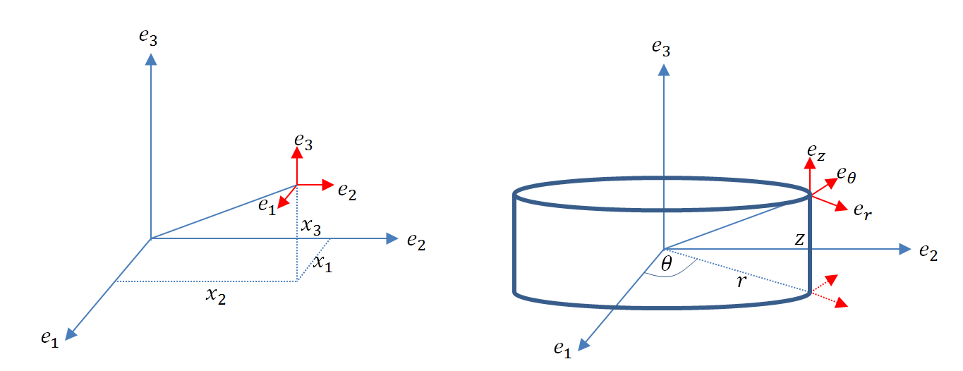
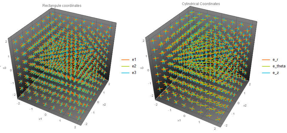
Cylindrical Coordinate System:
A cylindrical coordinate system is a system used for directions in \mathbb{R}^3 in which a polar coordinate system is used for the first plane (Fig 2 and Fig 3). The coordinate system directions can be viewed as three vector fields  , and
, and  such that:
![\[\begin{split} e_r&=\cos(\theta)e_1+\sin(\theta)e_2\\ e_\theta&=-\sin(\theta)e_1+\cos(\theta)e_2\\ e_z&=e_3 \end{split} \]](https://engcourses-uofa.ca/wp-content/ql-cache/quicklatex.com-42f259204b4cfb32afeb68247f3399dd_l3.png "Rendered by QuickLaTeX.com")
with and related to the coordinates and using the polar coordinate system relationships. The coordinate transformation from the Cartesian basis to the cylindrical coordinate system is described at every point using the matrix :
![\[ Q=\left(\begin{matrix}\cos(\theta)&\sin(\theta)&0\\-\sin(\theta)&\cos(\theta)&0\\0&0&1\end{matrix}\right) \]](https://engcourses-uofa.ca/wp-content/ql-cache/quicklatex.com-57d5dad712634870ad395bf6e0c38eb9_l3.png "Rendered by QuickLaTeX.com")
The vector fields and are functions of and their derivatives with respect to and follow from the polar coordinate system. on the other hand is independent of and .
Fields in Cylindrical Coordinate System
Let  be a subset of
  . If
. If  ,
,  , and
, and  are smooth scalar, vector and second-order tensor fields, then they can be chosen to be functions of either the Cartesian coordinates
  , and
, and  , or the corresponding real numbers , , and
  . Also,
  and
and  can have their components expressed in either the fixed orthonormal basis set
  , or can be expressed using the cylindrical coordinate system directions at every point. In other words, , as a vector field, can have the one of the following forms:
![\[\begin{split} u(x_1,x_2,x_3)&=u_1(x_1,x_2,x_3)e_1+u_2(x_1,x_2,x_3)e_2+u_3(x_1,x_2,x_3)e_3\\ &=u(r,\theta,z)\\ &=u_r(r,\theta,z)e_r(\theta)+u_\theta(r,\theta,z)e_\theta(\theta)+u_z(r,\theta,z)e_z \end{split} \]](https://engcourses-uofa.ca/wp-content/ql-cache/quicklatex.com-0fa90eab3a6e17ea210a10df671f0f12_l3.png "Rendered by QuickLaTeX.com")
where  , and
, and  are scalar fields. Similarly, , as a tensor field, can have one of the following forms:
![\[\begin{split} T(x_1,x_2,x_3)&=T_{11}(x_1,x_2,x_3)e_1\otimes e_1+T_{12}(x_1,x_2,x_3)e_1\otimes e_2+T_{13}(x_1,x_2,x_3)e_1\otimes e_3\\ & +T_{21}(x_1,x_2,x_3)e_2\otimes e_1+T_{22}(x_1,x_2,x_3)e_2\otimes e_2+T_{23}(x_1,x_2,x_3)e_2\otimes e_3\\ & +T_{31}(x_1,x_2,x_3)e_3\otimes e_1+T_{32}(x_1,x_2,x_3)e_3\otimes e_2+T_{33}(x_1,x_2,x_3)e_3\otimes e_3\\ &=T(r,\theta,z)\\ &=T_{rr}(r,\theta,z)e_r(\theta)\otimes e_r(\theta)+T_{r\theta}(r,\theta,z)e_r(\theta)\otimes e_\theta(\theta)+T_{rz}(r,\theta,z)e_r(\theta)\otimes e_z\\ & +T_{\theta r}(r,\theta,z)e_\theta(\theta)\otimes e_r(\theta)+T_{\theta \theta}(r,\theta,z)e_\theta(\theta)\otimes e_\theta(\theta)+T_{\theta z}(r,\theta,z)e_\theta(\theta)\otimes e_z\\ & +T_{zr}(r,\theta,z)e_z\otimes e_r(\theta)+T_{z\theta}(r,\theta,z)e_z\otimes e_\theta(\theta)+T_{zz}(r,\theta,z)e_z\otimes e_z \end{split} \]](https://engcourses-uofa.ca/wp-content/ql-cache/quicklatex.com-40a5bcfebbf20f7ca79a9e75f88d228b_l3.png "Rendered by QuickLaTeX.com")
where  , and
, and  are scalar fields.
Field Derivatives in Cylindrical Coordinate Systems
Gradient of a Scalare Field
Let  be a scalar field such that
  . The gradient of
  in a cylindrical coordinate system can be obtained using one of two ways. The first way is to find as a function of , and by simply replacing ,, and . Then, finding the gradient of in the Cartesian coordinate system and then utilizing the relationship
  . After that, the variables
  , and can be replaced with
  , and . Alternative, the gradient of can be obtained directly in the cylindrical coordinate system. In order to find the expression for the gradient, recall that a scalar field is differentiable if there exists
  such that
  ,
, 
![\[ \lim_{h\rightarrow 0}\left|\frac{\phi(x+hn)-\phi(x)}{h}-\nabla\phi\cdot n\right|=0 \]](https://engcourses-uofa.ca/wp-content/ql-cache/quicklatex.com-56267275bf6858e553ffd74ab2e78fbf_l3.png "Rendered by QuickLaTeX.com")
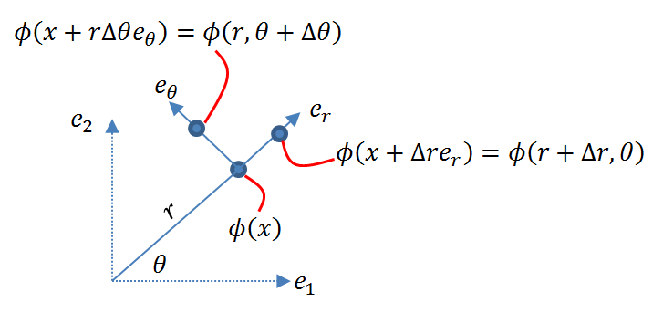
Using this definition, we will aim to find the representation of  in a cylindrical coordinate system. Let
  . We will strategically choose particular expressions for hn to obtain the required expression for the vector . First, we will choose hn such that it is equivalent to a path increment caused by a change \Delta r, i.e., hn=\Delta r \frac{\partial x}{\partial r}=\Delta r e_r (Fig. 4). Then:
![\[ \lim_{\Delta r\rightarrow 0}\left|\frac{\phi(x+\Delta r e_r)-\phi(x)}{\Delta r}-\nabla\phi\cdot e_r\right|=0 \]](https://engcourses-uofa.ca/wp-content/ql-cache/quicklatex.com-349d401146607d711ca8f42413ca0cf0_l3.png "Rendered by QuickLaTeX.com")
Therefore:
![\[ \lim_{\Delta r\rightarrow 0}\left|\frac{\phi(r+\Delta r,\theta,z)-\phi(r,\theta,z)}{\Delta r}\right|=\nabla\phi_r \]](https://engcourses-uofa.ca/wp-content/ql-cache/quicklatex.com-c52038e12009b55c2971d821d75b015c_l3.png "Rendered by QuickLaTeX.com")
Therefore:
![\[ \nabla \phi_r=\frac{\partial \phi}{\partial r} \]](https://engcourses-uofa.ca/wp-content/ql-cache/quicklatex.com-f88c05e572c28dc5a08e803407b55980_l3.png "Rendered by QuickLaTeX.com")
Similarly,  can be chosen to be equivalent to a path increment caused by
  , i.e.,
  (Fig. 4). Therefore:
![\[ \lim_{\Delta \theta \rightarrow 0}\left|\frac{\phi(x+r\Delta \theta e_\theta)-\phi(x)}{\Delta \theta}-\nabla\phi\cdot re_\theta\right|=0 \]](https://engcourses-uofa.ca/wp-content/ql-cache/quicklatex.com-f0c62021dd1129666c6bda02ff57cd0d_l3.png "Rendered by QuickLaTeX.com")
Therefore:
![\[ \lim_{\Delta \theta \rightarrow 0}\left|\frac{\phi(x+r\Delta \theta e_\theta)-\phi(x)}{\Delta \theta}\right|=\nabla\phi\cdot re_\theta=r\nabla\phi_\theta \]](https://engcourses-uofa.ca/wp-content/ql-cache/quicklatex.com-3334b895dc2e511d990775fb6f17f587_l3.png "Rendered by QuickLaTeX.com")
Therefore:
![\[ \lim_{\Delta \theta \rightarrow 0}\left|\frac{\phi(r,\theta+\Delta\theta,z)-\phi(r,\theta,z)}{\Delta \theta}\right|=r\nabla\phi_\theta \]](https://engcourses-uofa.ca/wp-content/ql-cache/quicklatex.com-58bb2b327ee57fc3116356427550c1b8_l3.png "Rendered by QuickLaTeX.com")
Therefore,
![\[ \nabla\phi_\theta=\frac{\partial \phi}{r\partial\theta} \]](https://engcourses-uofa.ca/wp-content/ql-cache/quicklatex.com-521949695115b88b1cc2e817ec0eab78_l3.png "Rendered by QuickLaTeX.com")
The third component is straightforward and is equal to:
![\[ \nabla\phi_z=\frac{\partial \phi}{\partial z} \]](https://engcourses-uofa.ca/wp-content/ql-cache/quicklatex.com-68d202ac027523c166a4890bd9a039de_l3.png "Rendered by QuickLaTeX.com")
Therefore, the gradient of in a cylindrical coordinate system has the form:
![\[ \nabla \phi = \frac{\partial \phi}{\partial r} e_r + \frac{\partial \phi}{r\partial \theta} e_\theta+ \frac{\partial \phi}{\partial z} e_z \]](https://engcourses-uofa.ca/wp-content/ql-cache/quicklatex.com-2e8059c93bedfcacc4ce9c802d0557dc_l3.png "Rendered by QuickLaTeX.com")
Gradient of a Vector Field
Let  be a smooth vector field. The components of the tensor field
  in a cylindrical coordinate system can be obtained by a simple coordinate transformation using the components in the Cartesian coordinate system and the matrix of transformation . I.e.,
  . Alternatively, if is already expressed in a cylindrical coordinate system, then, notice that the derivatives of with respect to , , and are given by:
![\[\begin{split} \frac{\partial u}{\partial r}&=\frac{\partial u_r}{\partial r}e_r+\frac{\partial u_\theta}{\partial r}e_\theta+\frac{\partial u_z}{\partial r}e_z\\ \frac{\partial u}{\partial \theta}&=\frac{\partial u_r}{\partial \theta}e_r+u_r e_\theta+\frac{\partial u_\theta}{\partial \theta}e_\theta-u_{\theta}e_r+\frac{\partial u_z}{\partial \theta}e_z\\ \frac{\partial u}{\partial z}&=\frac{\partial u_r}{\partial z}e_r+\frac{\partial u_\theta}{\partial z}e_\theta+\frac{\partial u_z}{\partial z}e_z \end{split} \]](https://engcourses-uofa.ca/wp-content/ql-cache/quicklatex.com-449586bae4d36c4faff44fd683a6e805_l3.png "Rendered by QuickLaTeX.com")
We can now assume assume that, in the cylindrical coordinate system,  has the following form:
![\[ \nabla u'=\left(\begin{matrix}\nabla u_{rr} & \nabla u_{r\theta} & \nabla u_{rz}\\ \nabla u_{\theta r} & \nabla u_{\theta \theta} & \nabla u_{\theta z}\\\nabla u_{zr} & \nabla u_{z\theta} & \nabla u_{zz} \end{matrix}\right) \]](https://engcourses-uofa.ca/wp-content/ql-cache/quicklatex.com-c804d0d565b5a460728d665e05940737_l3.png "Rendered by QuickLaTeX.com")
Notice that:
![\[\begin{split} \nabla u_{rr}&=\nabla u e_r\cdot e_r\\ \nabla u_{r\theta}&=\nabla u e_\theta \cdot e_r\\ \nabla u_{rz}&=\nabla u e_z \cdot e_r\\ \nabla u_{\theta r}&=\nabla u e_r\cdot e_\theta \\ \nabla u_{\theta \theta}&=\nabla u e_\theta \cdot e_\theta \\ \nabla u_{\theta z}&=\nabla u e_z \cdot e_\theta \\ \nabla u_{z r}&=\nabla u e_r\cdot e_z \\ \nabla u_{z \theta}&=\nabla u e_\theta \cdot e_z \\ \nabla u_{z z}&=\nabla u e_z \cdot e_z \end{split} \]](https://engcourses-uofa.ca/wp-content/ql-cache/quicklatex.com-49b8b88f9d807d341ad57b7f0fb62f7d_l3.png "Rendered by QuickLaTeX.com")
Recall that a vector field is differentiable if there exists a tensor field denoted such that  :
:
![\[ \lim_{h\rightarrow 0}\left\|\frac{u(x+hn)-u(x)}{h}-\nabla u(n)\right\|=0 \]](https://engcourses-uofa.ca/wp-content/ql-cache/quicklatex.com-e82916e75eb36aaa46a4d425d3d66ce4_l3.png "Rendered by QuickLaTeX.com")
Therefore, the component  can be obtained by setting
  in the above relationship and taking the dot product with as follows:
![\[ \lim_{\Delta r\rightarrow 0}\left(\frac{u(x+\Delta r e_r)-u(x)}{\Delta r}\right)\cdot e_r=\nabla u_{rr} \]](https://engcourses-uofa.ca/wp-content/ql-cache/quicklatex.com-df8e147994c21c028829711610deb130_l3.png "Rendered by QuickLaTeX.com")
I.e.
![\[ \frac{\partial u}{\partial r}\cdot e_r=\nabla u_{rr} \]](https://engcourses-uofa.ca/wp-content/ql-cache/quicklatex.com-5abf5956fcce147d0f6d98ded077fbc7_l3.png "Rendered by QuickLaTeX.com")
Therefore:
![\[ \nabla u_{rr}=\frac{\partial u_r}{\partial r} \]](https://engcourses-uofa.ca/wp-content/ql-cache/quicklatex.com-5ffa04e7a3972db39599c822d29683aa_l3.png "Rendered by QuickLaTeX.com")
The component  can be obtained by setting
  in the above relationship and taking the dot product with as follows:
![\[ \lim_{\Delta \theta\rightarrow 0}\left(\frac{u(x+r\Delta \theta e_\theta)-u(x)}{\Delta \theta}\right)\cdot e_r=r\nabla u_{r\theta} \]](https://engcourses-uofa.ca/wp-content/ql-cache/quicklatex.com-710f04fde0a526430b1e17f3a376c4d8_l3.png "Rendered by QuickLaTeX.com")
I.e.
![\[ \frac{\partial u}{\partial \theta}\cdot e_r=r\nabla u_{r\theta} \]](https://engcourses-uofa.ca/wp-content/ql-cache/quicklatex.com-e83dd7c89325149ae0c90a08c7b4df2f_l3.png "Rendered by QuickLaTeX.com")
Therefore:
![\[ \nabla u_{r\theta}=\frac{\partial u}{r\partial \theta}\cdot e_r=\frac{\partial u_r}{r\partial \theta}-\frac{u_{\theta}}{r} \]](https://engcourses-uofa.ca/wp-content/ql-cache/quicklatex.com-c154dda872dad67465f0065dfefa1a0a_l3.png "Rendered by QuickLaTeX.com")
Similarly,
![\[\begin{split} \nabla u_{\theta r}&=\frac{\partial u_\theta}{\partial r}\\ \nabla u_{\theta \theta}&=\frac{\partial u_\theta}{r\partial \theta}+\frac{u_r}{r}\\ \nabla u_{\theta z}&=\frac{\partial u_\theta}{\partial z}\\ \nabla u_{z \theta}&=\frac{\partial u_z}{r\partial \theta}\\ \nabla u_{rz}&=\frac{\partial u_r}{\partial z}\\ \nabla u_{z r}&=\frac{\partial u_z}{\partial r}\\ \nabla u_{zz}&=\frac{\partial u_z}{\partial z} \end{split} \]](https://engcourses-uofa.ca/wp-content/ql-cache/quicklatex.com-7a6052edf8b96fc22643164918eb99ac_l3.png "Rendered by QuickLaTeX.com")
Therefore, has the following form:
![\[ \nabla u'=\left(\begin{matrix} \frac{\partial u_r}{\partial r} & \frac{\partial u_r}{r\partial \theta}-\frac{u_{\theta}}{r} &\frac{\partial u_r}{\partial z}\\ \frac{\partial u_\theta}{\partial r} & \frac{\partial u_\theta}{r\partial \theta}+\frac{u_r}{r} &\frac{\partial u_\theta}{\partial z}\\ \frac{\partial u_z}{\partial r} & \frac{\partial u_z}{r\partial \theta}& \frac{\partial u_z}{\partial z} \end{matrix}\right) \]](https://engcourses-uofa.ca/wp-content/ql-cache/quicklatex.com-8f4d8eda15111fb04039b9bf0b0c3bc4_l3.png "Rendered by QuickLaTeX.com")
Divergence of a Vector Field
If is given similar to the previous section, then, the divergence of in a cylindrical coordinate system is given by:
![\[ \mathrm{div}(u)=\mathrm{Trace}(\nabla u)=\frac{\partial u_r}{\partial r}+\frac{\partial u_\theta}{r\partial \theta}+\frac{u_r}{r}+\frac{\partial u_z}{\partial z} \]](https://engcourses-uofa.ca/wp-content/ql-cache/quicklatex.com-f47561b4a92de413e3cc2eb66fc9ee0a_l3.png "Rendered by QuickLaTeX.com")
Gradient of a Tensor Field
Let  be a tensor field with components
  with
with  . First, we use the tensor product representation of the tensor field to find the derivatives of with respect to , and . The derivatives with respect to and are straightforward since
  , and are independent of and :
![\[\begin{split} \frac{\partial T(r,\theta,z)}{\partial r}=&\frac{\partial T_{rr}}{\partial r}e_r\otimes e_r+\frac{\partial T_{r\theta}}{\partial r}e_r\otimes e_\theta+\frac{\partial T_{rz}}{\partial r}e_r\otimes e_z\\ & +\frac{\partial T_{\theta r}}{\partial r}e_\theta\otimes e_r+\frac{\partial T_{\theta\theta}}{\partial r}e_\theta\otimes e_\theta+\frac{\partial T_{\theta z}}{\partial r}e_\theta\otimes e_z\\ & +\frac{\partial T_{zr}}{\partial r}e_z\otimes e_r+\frac{\partial T_{z\theta}}{\partial r}e_z\otimes e_\theta+\frac{\partial T_{zz}}{\partial r}e_z\otimes e_z \end{split} \]](https://engcourses-uofa.ca/wp-content/ql-cache/quicklatex.com-b93d9ef5dd6f4088eb6ab2c54b40cb3f_l3.png "Rendered by QuickLaTeX.com")
Similarly,
![\[\begin{split} \frac{\partial T(r,\theta,z)}{\partial z}=&\frac{\partial T_{rr}}{\partial z}e_r\otimes e_r+\frac{\partial T_{r\theta}}{\partial z}e_r\otimes e_\theta+\frac{\partial T_{rz}}{\partial z}e_r\otimes e_z\\ & +\frac{\partial T_{\theta r}}{\partial z}e_\theta\otimes e_r+\frac{\partial T_{\theta\theta}}{\partial z}e_\theta\otimes e_\theta+\frac{\partial T_{\theta z}}{\partial z}e_\theta\otimes e_z\\ & +\frac{\partial T_{zr}}{\partial z}e_z\otimes e_r+\frac{\partial T_{z\theta}}{\partial z}e_z\otimes e_\theta+\frac{\partial T_{zz}}{\partial z}e_z\otimes e_z \end{split} \]](https://engcourses-uofa.ca/wp-content/ql-cache/quicklatex.com-2ebc0859b11796ac0c5ed47aee24ee22_l3.png "Rendered by QuickLaTeX.com")
However, the dependence of and  on leads to the following derivative of with respect to :
![\[ \begin{split} \frac{\partial T(r,\theta,z)}{\partial \theta}=&\frac{\partial T_{rr}}{\partial \theta}e_r\otimes e_r+\frac{\partial T_{r\theta}}{\partial \theta}e_r\otimes e_\theta+\frac{\partial T_{rz}}{\partial \theta}e_r\otimes e_z\\ & +\frac{\partial T_{\theta r}}{\partial \theta}e_\theta\otimes e_r+\frac{\partial T_{\theta\theta}}{\partial \theta}e_\theta\otimes e_\theta+\frac{\partial T_{\theta z}}{\partial \theta}e_\theta\otimes e_z\\ & +\frac{\partial T_{zr}}{\partial \theta}e_z\otimes e_r+\frac{\partial T_{z\theta}}{\partial \theta}e_z\otimes e_\theta+\frac{\partial T_{zz}}{\partial \theta}e_z\otimes e_z\\ &+T_{rr}e_r\otimes e_\theta+T_{rr}e_\theta\otimes e_r-T_{r\theta}e_r\otimes e_r+T_{r\theta}e_\theta\otimes e_\theta+T_{rz}e_\theta\otimes e_z\\ &+T_{\theta r}e_\theta\otimes e_\theta-T_{\theta r}e_r\otimes e_r-T_{\theta\theta}e_\theta\otimes e_r-T_{\theta\theta}e_r\otimes e_\theta-T_{\theta z}e_r\otimes e_z\\ &+T_{z r}e_z\otimes e_\theta-T_{z\theta}e_z\otimes e_r \end{split} \]](https://engcourses-uofa.ca/wp-content/ql-cache/quicklatex.com-67f768becb272af6c926b4d33fea6a11_l3.png "Rendered by QuickLaTeX.com")
Using the general definition of the gradient of a tensor field, the components of the gradient of denoted by  in the cylindrical coordinate system can be obtained in a manner similar to the previous section. Let the components be
  with
with  . Then, it is straightforward (but with lots of details) to show that when
  or
or  :
:
![\[ (\nabla T)_{\alpha \beta \gamma}=\left(\frac{\partial T}{\partial \gamma}e_{\beta}\right)\cdot e_\alpha \]](https://engcourses-uofa.ca/wp-content/ql-cache/quicklatex.com-3bed68579871a7828ba816c01c051539_l3.png "Rendered by QuickLaTeX.com")
Therefore:
![\[\begin{split} (\nabla T)_{\alpha\beta r}=&\frac{\partial T_{\alpha \beta}}{\partial r}\\ (\nabla T)_{\alpha\beta z}=&\frac{\partial T_{\alpha \beta}}{\partial z} \end{split} \]](https://engcourses-uofa.ca/wp-content/ql-cache/quicklatex.com-fba8e649362f9965b77e8f8a2192a89c_l3.png "Rendered by QuickLaTeX.com")
However, the components when \gamma=\theta have the following form:
![\[ \begin{split} (\nabla T)_{rr\theta}=&\frac{\partial T_{rr}}{r\partial \theta}-\frac{T_{r\theta}}{r}-\frac{T_{\theta r}}{r}\\ (\nabla T)_{r\theta\theta}=&\frac{\partial T_{r\theta}}{r\partial \theta}+\frac{T_{rr}}{r}-\frac{T_{\theta \theta}}{r}\\ (\nabla T)_{rz\theta}=&\frac{\partial T_{rz}}{r\partial \theta}-\frac{T_{\theta z}}{r}\\ (\nabla T)_{\theta r\theta}=&\frac{\partial T_{\theta r}}{r\partial \theta}+\frac{T_{rr}}{r}-\frac{T_{\theta \theta}}{r}\\ (\nabla T)_{\theta \theta \theta}=&\frac{\partial T_{\theta \theta}}{r\partial \theta}+\frac{T_{r\theta}}{r}+\frac{T_{\theta r}}{r}\\ (\nabla T)_{\theta z\theta}=&\frac{\partial T_{\theta z}}{r\partial \theta}+\frac{T_{rz}}{r}\\ (\nabla T)_{zr\theta}=&\frac{\partial T_{zr}}{r\partial \theta}-\frac{T_{z\theta}}{r}\\ (\nabla T)_{z \theta \theta}=&\frac{\partial T_{z\theta}}{r\partial \theta}+\frac{T_{zr}}{r}\\ (\nabla T)_{zz\theta}=&\frac{\partial T_{zz}}{r\partial \theta}\\ \end{split} \]](https://engcourses-uofa.ca/wp-content/ql-cache/quicklatex.com-cbb2c2ab3cade36c342674258c6ff0d2_l3.png "Rendered by QuickLaTeX.com")
Divergence of a Tensor Field
Let be a tensor field with the cylindrical coordinate system components  with .
Using the general definition of the divergence of a tensor field, the components of \mathrm{div}{(T)} in a cylindrical coordinate system can be obtained as follows:
![\[\begin{split} (\mathrm{div}(T))_r=&\mathrm{div}(Te_r)=\mathrm{Trace}(\nabla T e_r)\\ (\mathrm{div}(T))_\theta=&\mathrm{div}(Te_\theta)=\mathrm{Trace}(\nabla T e_\theta)\\ (\mathrm{div}(T))_z=&\mathrm{div}(Te_z)=\mathrm{Trace}(\nabla T e_z) \end{split} \]](https://engcourses-uofa.ca/wp-content/ql-cache/quicklatex.com-881f042732597803e6a8ca8b8ad7872f_l3.png "Rendered by QuickLaTeX.com")
where , and are fixed in space at a particular point. I.e., the  operator only applies to . The procedure used in the gradient of a vector in a cylindrical coordinate system section combined with the derivatives of shown in the previous section can be used to reach the following formulas for the components of the divergence of in a cylindrical coordinate system:
![\[\begin{split} \mathrm{div}{(T)}&=\left(\begin{array}{c} \mathrm{Trace}(\nabla Te_r)\\\mathrm{Trace}(\nabla Te_\theta)\\\mathrm{Trace}(\nabla Te_z)\end{array}\right)\\ &=\left(\begin{array}{c} \left(\frac{\partial T}{\partial r}e_r \right)\cdot e_r + \left(\frac{\partial T}{r\partial \theta}e_r \right)\cdot e_\theta + \left(\frac{\partial T}{\partial z}e_r \right)\cdot e_z\\ \left(\frac{\partial T}{\partial r}e_\theta \right)\cdot e_r + \left(\frac{\partial T}{r\partial \theta}e_\theta \right)\cdot e_\theta + \left(\frac{\partial T}{\partial z}e_\theta \right)\cdot e_z\\ \left(\frac{\partial T}{\partial r}e_z \right)\cdot e_r + \left(\frac{\partial T}{r\partial \theta}e_z \right)\cdot e_\theta + \left(\frac{\partial T}{\partial z}e_z \right)\cdot e_z\end{array}\right)\\ &=\left(\begin{array}{c} \sum_{\alpha\in\{r,\theta,z\}}(\nabla T)_{\alpha r r}\\ \sum_{\alpha\in\{r,\theta,z\}}(\nabla T)_{\alpha \theta \theta} \\ \sum_{\alpha\in\{r,\theta,z\}}(\nabla T)_{\alpha z z}\end{array}\right) \end{split} \]](https://engcourses-uofa.ca/wp-content/ql-cache/quicklatex.com-66d0ae47e588a09de799b5991ea525c1_l3.png "Rendered by QuickLaTeX.com")
Therefore:
![\[ \mathrm{div}{(T)}=\left(\begin{array}{c} \frac{\partial T_{rr}}{\partial r}+\frac{\partial T_{r\theta}}{r\partial \theta}+\frac{T_{rr}-T_{\theta\theta}}{r}+\frac{\partial T_{rz}}{\partial z}\\ \frac{\partial T_{\theta r}}{\partial r}+\frac{\partial T_{\theta\theta}}{r\partial \theta}+\frac{T_{r\theta}+T_{\theta r}}{r}+\frac{\partial T_{\theta z}}{\partial z}\\ \frac{\partial T_{zr}}{\partial r}+\frac{\partial T_{z\theta}}{r\partial \theta}+\frac{T_{zr}}{r}+\frac{\partial T_{z z}}{\partial z} \end{array} \right) \]](https://engcourses-uofa.ca/wp-content/ql-cache/quicklatex.com-63a2048c797e10677bd3c914fb3a6235_l3.png "Rendered by QuickLaTeX.com")
Curl of a Vector Field
Using the general definition of the Curl, if is a vector field given in terms of , and and represented in a cylindrical coodrinate system, then, the components of the curl of are given by:
![\[\begin{split} (\mbox{curl}(u))_r&=(\mbox{curl}(u))\cdot e_r=\mbox{div}(u\times e_r)=\mbox{Trace}(\nabla u\times e_r)\\ (\mbox{curl}(u))_\theta&=(\mbox{curl}(u))\cdot e_\theta=\mbox{div}(u\times e_\theta)=\mbox{Trace}(\nabla u\times e_\theta)\\ (\mbox{curl}(u))_z&=(\mbox{curl}(u))\cdot e_z=\mbox{div}(u\times e_z)=\mbox{Trace}(\nabla u\times e_z) \end{split} \]](https://engcourses-uofa.ca/wp-content/ql-cache/quicklatex.com-7f2c507eee0d1d65e2b9029add60ea03_l3.png "Rendered by QuickLaTeX.com")
with the \nabla operator applied to u and not to the vectors , and . Therefore in a cylindrical coordinate system:
![\[ \mbox{curl}(u)=\left(\begin{array}{c}\frac{\partial u_z}{r\partial \theta}-\frac{\partial u_{\theta}}{\partial z}\\ \frac{\partial u_r}{\partial z}-\frac{\partial u_z}{\partial r}\\ \frac{\partial u_\theta}{\partial r}+\frac{u_{\theta}}{r}-\frac{\partial u_r}{r\partial \theta} \end{array}\right) \]](https://engcourses-uofa.ca/wp-content/ql-cache/quicklatex.com-de3e4441cc332d7b32bfb97e17905b2c_l3.png "Rendered by QuickLaTeX.com")
Laplacian of a Scalar Field
Using the general definition of the Laplacian, if is a scalar function given in terms of , and , then, the Laplacian of is given by:
![\[\begin{split} \nabla^2\phi&=\mathrm{div}(\nabla \phi)\\ &=\mathrm{div}\left(\frac{\partial \phi}{\partial r} e_r + \frac{\partial \phi}{r\partial \theta} e_\theta+ \frac{\partial \phi}{\partial z} e_z\right)\\ &=\frac{\partial^2 \phi}{\partial r^2}+\frac{\partial^2 \phi}{r^2\partial \theta^2}+\frac{\partial \phi}{r\partial r}+\frac{\partial^2 \phi}{\partial z^2} \end{split} \]](https://engcourses-uofa.ca/wp-content/ql-cache/quicklatex.com-edd4cc68fd2006398f15c06424624a79_l3.png "Rendered by QuickLaTeX.com")
Example
Let  be given by
  . Find the gradient of in the current coordinate system. Find the expression for and the gradient of in a polar coordinate system.
SOLUTION
In the Cartesian coordinate system, the gradient of has the form:
![\[ \nabla u=\left(\begin{matrix}2x_1&2x_2\\x_2&x_1\end{matrix}\right) \]](https://engcourses-uofa.ca/wp-content/ql-cache/quicklatex.com-462e85abccd62a40fbe3485424b28633_l3.png "Rendered by QuickLaTeX.com")
Note that and can be represented in the Cartesian coordinate system using and instead of and as follows:
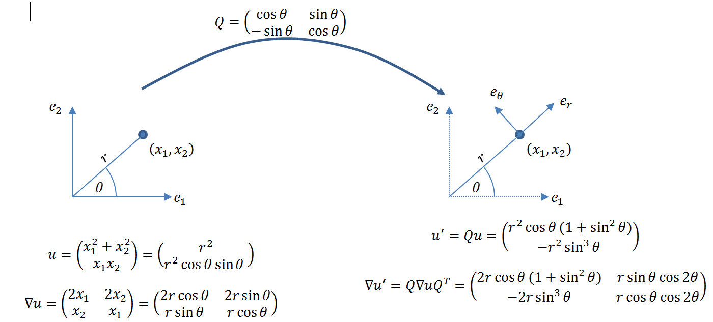
![\[ \begin{split} u=&\left(\begin{array}{c}r^2\\r^2\cos(\theta)\sin(\theta)\end{array}\right)\\ \nabla u=&\left(\begin{matrix}2r\cos(\theta)&2r\sin(\theta)\\r\sin(\theta)&r\cos(\theta)\end{matrix}\right) \end{split} \]](https://engcourses-uofa.ca/wp-content/ql-cache/quicklatex.com-187fb00107a578ebd411b7bd7c45c0bb_l3.png "Rendered by QuickLaTeX.com")
It is important to note that this is a mere change of variables, but the components of and are still represented using the Cartesian coordinate system. The values themselves are just obtained using and , rather than and .
If , and are the basis vectors in the Cartesian coordinate system, and if and are the basis vectors in the cylindrical coordinate system, then the matrix of transformation from the Cartesian to the cylindrical coordinate system at a particular point depends on the value of theta at that particular point and is given by:
If  is the expression of in the polar coordinate system, it has the form:
![\[ u'=Qu=\left(\begin{array}{c}u_r\\u_\theta\end{array}\right)=\left(\begin{array}{c}r^2\cos(\theta)\left(1+\sin^2(\theta)\right)\\-r^2\sin^3(\theta)\end{array}\right) \]](https://engcourses-uofa.ca/wp-content/ql-cache/quicklatex.com-7a87c39b396f2ca820e952e4f3971456_l3.png "Rendered by QuickLaTeX.com")
The representation in the cylindrical coordinate system can be obtained using the change of coordinates formula:
![\[ \nabla u'=Q\nabla u Q^T=\left(\begin{matrix}-r\cos(\theta)(-3+\cos(2\theta))&r\cos(2\theta)\sin(\theta)\\-2r\sin^3(\theta)&r\cos(2\theta)\cos(\theta)\end{matrix}\right) \]](https://engcourses-uofa.ca/wp-content/ql-cache/quicklatex.com-dc82b4701c5f0ab91834ba6ce283ee02_l3.png "Rendered by QuickLaTeX.com")
Alternatively, the gradient of u in the cylindrical coordinate system can be obtained directly using the components  and
and  :
:
![\[ \nabla u'=\left(\begin{matrix} \frac{\partial u_r}{\partial r} & \frac{\partial u_r}{r\partial \theta}-\frac{u_{\theta}}{r} \\ \frac{\partial u_\theta}{\partial r} & \frac{\partial u_\theta}{r\partial \theta}+\frac{u_r}{r} \end{matrix}\right)= \left(\begin{matrix}2r\cos(\theta)(1+\sin^2(\theta))&r\cos(2\theta)\sin(\theta)\\-2r\sin^3(\theta)&r\cos(2\theta)\cos(\theta)\end{matrix}\right) \]](https://engcourses-uofa.ca/wp-content/ql-cache/quicklatex.com-856ad0699e5fe75330898ab458abfcf9_l3.png "Rendered by QuickLaTeX.com")
Noting that  , the two methods produce identical results for the components of the gradient in the polar coordinate system.
The following figure shows the directions at an arbitrary point  in a Cartesian coordinate system (left) and the representation of and in that coordinate system. On the right, the polar coordinate system directions are shown along with the representation and .
View Mathematica Code
Q={{Cos[th],Sin[th]},{-Sin[th],Cos[th]}};
u={x1^2+x2^2,x1*x2};
x={x1,x2}
rule={x1->r*Cos[th],x2->r*Sin[th]}
urth=FullSimplify[u/.rule]
Gu=Table[D[u[[i]],x[[j]]],{i,1,2},{j,1,2}]
Gurth=FullSimplify[Gu/.rule]
up=FullSimplify[Q.urth]
Gup=FullSimplify[Q.Gurth.Transpose[Q]]
Gup//MatrixForm
Guformula=FullSimplify[{{D[up[[1]],r],D[up[[1]],th]/r-up[[2]]/r},{D[up[[2]],r],up[[1]]/r+D[up[[2]],th]/r}}];
Guformula//MatrixForm
FullSimplify[Guformula-Gup]
View Python Code
import sympy as sp
from sympy import diff, simplify
from sympy.matrices import Matrix
sp.init_printing(use_latex = "mathjax")
x1,x2 = sp.symbols('x_1 x_2')
r, theta = sp.symbols('r \u03B8')
u1 = x1**2+x2**2
u2 = x1*x2
# cartesian coordinate system
u = Matrix([u1,u2])
display("u =",u)
x=Matrix([x1,x2])
# gradient
grad_u=Matrix([[diff(ui,xj) for xj in x] for ui in u])
display("\u2207u =",grad_u)
# Change of variables
display("The following is a simple change of variables but the components are still in the cartesian coordinate system")
urth = u.subs([(x1, r*sp.cos(theta)), (x2, r*sp.sin(theta))])
display("u_r_\u03B8 =",urth,simplify(urth))
# gradient
grad_u_rth = grad_u.subs([(x1, r*sp.cos(theta)), (x2, r*sp.sin(theta))])
display("\u2207u_r_\u03B8 =",grad_u_rth)
# rot matrix
Q = Matrix([[sp.cos(theta),sp.sin(theta)],[-sp.sin(theta),sp.cos(theta)]])
display("Q =",Q)
# Change of coordinates
display("The following representation is in the radial coordinate system")
upolar=simplify(Q*urth)
grad_u_polar=simplify(Q*grad_u_rth*Q.T)
display("u' = Q*u =",upolar)
display("\u2207u' = Q*\u2207u*Q^T =",grad_u_polar)
# Gradient formula in the polar coordinate system
display("The gradient can also be calculated using the gradient formula")
grad_u_formula=Matrix([[diff(upolar[0],r),diff(upolar[0],theta)/r-upolar[1]/r],
                [diff(upolar[1],r),upolar[0]/r+diff(upolar[1],theta)/r]])
grad_u_formula=simplify(grad_u_formula)
display(grad_u_formula)