Engineering at Alberta Courses » The Weighted Residuals Method

Approximate Methods: The Weighted Residuals Method

The statement of the equilibrium equations applied to a set $D\subset\mathbb{R}^3$ is as follows. Assuming that at equilibrium $\sigma:D\rightarrow\mathbb{M}^3$ is the symmetric Cauchy stress distribution on $D$ and that $u:D\rightarrow\mathbb{R}^3$ is the displacement vector distribution and knowing the relationship $\sigma=\sigma(u)$ , then the equilibrium equation seeks to find $u\in U$ such that the associated \sigma satisfies the equation:

$\mathrm{div}\sigma+\rho b= 0$

where $b:D\rightarrow\mathbb{R}^3$ is the body forces vector distribution on $D$ , $\rho$ is the mass density, and $U$ is the space of all possible displacement functions applied to $D$ , i.e., $U=\{a:D\rightarrow\mathbb{R}^3| a\mbox{ is kinematically admissible}\}$ . The term “Kinematically admissible” in $U$ indicates that the space of possible solutions must satisfy the boundary conditions imposed on $\partial D_u$ (as stated below) and any differentiability constraints.

The boundary conditions for the equations of equilibrium are usually given on two parts of the boundary of $D$ denoted $\partial D$ . On the first part, $\partial D_n$ , the external traction vectors $t_n$ are known so we have the boundary conditions for $\sigma$ since $\sigma^Tn=t_n$ ( $n$ is the normal vector to the boundary). On the second part, $\partial D_u$ , the displacement is given.

The weighted residuals method seeks an approximate solution $u_{approx}$ with a particular form that has a finite number of unknown parameters. Since $u_{approx}$ does not necessarily satisfy the requirements for the problem, the corresponding stresses $\sigma_{approx}$ would not satisfy equilibrium. The residuals $R$ are defined as the resulting values when the approximate solutions are substituted in the differential equation:

$R=\mathrm{div}\sigma_{approx}+\rho b$

If $m$ is the number of unknown parameters in $u_{approx}$ then $m$ weight functions $W_i$ can be chosen. For each $i\leq m$ , an integral form of the residuals is set to zero:

(1) $\begin{equation*} \int_{D} \! RW_i \,\mathrm{d}x=0 \end{equation*}$

The form of $u_{approx}$ should be chosen satisfying the essential boundary conditions while the non-essential boundary conditions can be imposed in a variety of ways. There are two ways that the non-essential boundary conditions can be imposed. In the first one, if $D_su-g=0$ is the imposed boundary conditions on the boundary $\partial D_n$ , then, the residual $R_n=D_su_{approx}-g$ is first defined and the boundary condition is incorporated by setting

$\int_{\partial D_n} \! R_nW_i \,\mathrm{d}s=0$

Alternatively, the non-essential boundary conditions are incorporated directly in Equation 1 using integration by parts as will be shown later.

The Weighted Residuals Methods

Assuming $u_{approx}=a_0+a_1\phi_1(x)+a_2\phi_2(x)+a_3\phi_3(x)+\cdots + a_m\phi_m(x)$ , where $\forall i\leq m:\phi_i(x)$ is a known function and $a_i$ is an unknown parameters, the weighted residuals methods vary in the choice of the weight functions $W_i$ . The following is a list of possible choices for $W_i$ :

Least Squares Method

In the least squares method, the weight functions $W_i$ is chosen such that

$W_i=\frac{\partial R}{\partial a_i}$

The least squares method is effectively minimizing the squares of the residuals:

$I=\int_{D} \! R^2 \,\mathrm{d}x=\mbox{minimum}$

Point Collocation Method

The Point Collocation Method described before is a special case where $m$ points are chosen such that $\forall i\leq m:x_i\in D$ and the weight functions are chosen such that $\forall i\leq m$ :

$W_i=\delta_{x_i}=\bigg\{ \begin{matrix}1 & x=x_i\\ 0 & \mbox{otherwise} \end{matrix}$

Sub-Domain Method

In this method, $m$ sub-domains are chosen such that $\forall i\leq m: D_i\in D$ and the weight functions are chosen such that $\forall i\leq m$ :

$W_i=\mathcal{X}_{D_i}=\bigg\{ \begin{matrix}1 & x\in D_i\\ 0 & \mbox{otherwise} \end{matrix}$

Galerkin Method

In the Galerkin method, the weight functions $W_i$ is chosen such that

$W_i=\phi_i(x)$

The Galerkin method is effectively the virtual work method.

Example

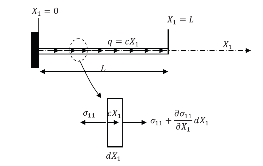
Using a polynomial trial function of the third degree, find the displacement function of the shown bar using the Galerkin method. Assume that the bar is linear elastic with Young’s modulus E and cross-sectional area A and that the small strain tensor is the appropriate measure of strain. Ignore the effect of Poisson’s ratio.

Solution

Exact Solution

The exact solution can be obtained by directly solving the differential equation of equilibrium utilizing $\sigma_{11}=E\frac{\mathrm{d}u_1}{\mathrm{d}X_1}$ :

$\frac{\mathrm{d}^2u_1}{\mathrm{d}X_1^2}=-\frac{cX_1}{EA}$

with the boundary conditions: $@X_1=0:u_1=0 and X_1=L:\frac{\mathrm{d}u_1}{\mathrm{d}X_1}=0$ . Therefore:

$u_1=\frac{cL^2}{2EA}X_1-\frac{c}{6EA}X_1^3$

View Mathematica Code

DSolve[{u''[X1] == -c*X1/EA, u'[L] == 0, u[0] == 0}, u[X1], X1]

View Python Code

from sympy import *
import sympy as sp 
sp.init_printing(use_latex = "mathjax")
u, c, EA, x, L = symbols("u c EA x L")
u = Function("u")
u1 = u(x).subs(x,0)
u2 = u(x).diff(x).subs(x,L)
sol = dsolve(u(x).diff(x,2)+c*x/EA, u(x), ics = {u1:0, u2:0})
display(sol)

Approximation Solution

The approximate solution has the form:

$u_{approx}=a_0+a_1X_1+a_2X_1^2+a_3X_1^3$

There is one essential boundary condition which is $@X_1=0:u_{approx}=0$ , therefore, $a_0=0$ . The approximate solution thus has the following form which satisfies the essential boundary conditions:

$u_{approx}=a_1X_1+a_2X_1^2+a_3X_1^3$

where $\phi_1(X_1)=X_1, \phi_2(X_1)=X_1^2$ , and $\phi_3(X_1)=X_1^3$ are the known functions and $a_1, a_2$ , and $a_3$ are the unknown parameters. The residuals have the form:

$R=\frac{\mathrm{d}^2u_{approx}}{\mathrm{d}X_1^2}+\frac{cX_1}{EA}$

The Galerkin method aims at setting the weighted residuals to zero:

$\int_{D} \! RW_i \,\mathrm{d}x= \int_{D} \! \left(\frac{\mathrm{d}^2u_{approx}}{\mathrm{d}X_1^2}+\frac{cX_1}{EA}\right)W_i \,\mathrm{d}x=0$

Rearranging:

$\int_0^L \! W_i\left(\frac{\mathrm{d}^2u_{approx}}{\mathrm{d}X_1^2}\right) \,\mathrm{d}X_1=\int_0^L \! -W_i\left(\frac{cX_1}{EA}\right) \,\mathrm{d}X_1$

Integration by parts of the left hand side can be used to incorporate the nonessential boundary conditions $\left(\frac{\mathrm{d}u_{approx}}{\mathrm{d}X_1}\right)\bigg|_{X_1=L}=0$ as follows:

$\begin{split} \int_0^L \! W_i\left(\frac{\mathrm{d}^2u_{approx}}{\mathrm{d}X_1^2}\right) \,\mathrm{d}X_1 & =W_i\left(\frac{\mathrm{d}u_{approx}}{\mathrm{d}X_1}\right)\bigg|_{X_1=0}^{X_1=L}-\int_0^L \! \frac{\mathrm{d}W_i}{\mathrm{d}X_1}\left(\frac{\mathrm{d}u_{approx}}{\mathrm{d}X_1}\right) \,\mathrm{d}X_1\\ &=0-\int_0^L \! \frac{\mathrm{d}W_i}{\mathrm{d}X_1}\left(\frac{\mathrm{d}u_{approx}}{\mathrm{d}X_1}\right) \,\mathrm{d}X_1 \end{split}$

Therefore, the Galerkin method equations now have the form:

$\int_0^L \! \frac{\mathrm{d}W_i}{\mathrm{d}X_1}\left(\frac{\mathrm{d}u_{approx}}{\mathrm{d}X_1}\right) \,\mathrm{d}X_1=\int_0^L \! W_i\left(\frac{cX_1}{EA}\right) \,\mathrm{d}X_1$

To find the unknowns $a_1, a_2$ , and $a_3$ , three equations are formed with $W_1=\phi_1(X_1)=X_1, W_2=\phi_2(X_1)=X_1^2$ , and $W_3=\phi_3(X_1)=X_1^3$ . Solving those three equations the following approximate solution is obtained:

$u_{approx}=\frac{cL^2}{2EA}X_1-\frac{c}{6EA}X_1^3$

Notice that since the exact solution (a polynomial of the third degree) is an element of the space of possible approximate solutions, the Galerkin method yields the exact solution!