
Linear Maps Between Vector Spaces: Examples and Problems
Examples and Problems
Example 1
Consider the symmetric matrix:
![\[ M=\left(\begin{matrix}1&1&0\\1&1&0\\0&0&1\end{matrix}\right) \]](https://engcourses-uofa.ca/wp-content/ql-cache/quicklatex.com-24f78f677770a87684f246f9c60f8004_l3.png "Rendered by QuickLaTeX.com")
Find  , the determinant of
  , the kernel of , the eigenvalues and eigenvectors of , and find the coordinate transformation in which is diagonal.
Solution
Since is symmetric, therefore,  . The determinant of can be obtained using the triple product of the row vectors. However, it is obvious that the first two vectors are linearly dependent (they are equal), therefore,
  . The kernel of can be obtained by finding the possible forms for the vector
  that would satisfy the following equation:
![\[ Mx=0\Rightarrow\left(\begin{matrix}1&1&0\\1&1&0\\0&0&1\end{matrix}\right)\left(\begin{array}{c}x_1\\x_2\\x_3\end{array}\right)=0 \]](https://engcourses-uofa.ca/wp-content/ql-cache/quicklatex.com-9b272913dfbb8745fb0b39fab4c36f17_l3.png "Rendered by QuickLaTeX.com")
Therefore:
![\[ x_1+x_2=0\qquad x_1+x_2=0\qquad x_3=0 \]](https://engcourses-uofa.ca/wp-content/ql-cache/quicklatex.com-cd2a7a2f5906239d649070bb78f9a183_l3.png "Rendered by QuickLaTeX.com")
By setting  , we have
  . Therefore, the kernel of has the form:
![\[ \ker{M}=\left\{x=\left(\begin{array}{c}\alpha\\-\alpha\\0\end{array}\right)\bigg| \alpha\in\mathbb{R}\right\} \]](https://engcourses-uofa.ca/wp-content/ql-cache/quicklatex.com-d9a0b733d826d1ca42f54a243d2ff01b_l3.png "Rendered by QuickLaTeX.com")
To find the eigenvalues of we find the possible values for  that would make the matrix
  not invertible. In other words, we solve for that would satisfy:
![\[ \det{M-\lambda I}=0\Rightarrow \det\left(\begin{matrix}1-\lambda&1&0\\1&1-\lambda&0\\0&0&1-\lambda\end{matrix}\right)=0 \]](https://engcourses-uofa.ca/wp-content/ql-cache/quicklatex.com-b27ad946c5fea7062e1e3e8b318e7416_l3.png "Rendered by QuickLaTeX.com")
Therefore:
![\[ (1-\lambda)^3-(1-\lambda)=0\Rightarrow \lambda^3-3\lambda^2+2\lambda=0\Rightarrow \lambda (\lambda -2)(\lambda -1)=0 \]](https://engcourses-uofa.ca/wp-content/ql-cache/quicklatex.com-22b86b0263e3e5c28cf40348038766c1_l3.png "Rendered by QuickLaTeX.com")
Therefore, the possible three eigenvalues are:  , and
, and  . Note that since is not invertible,
  is automatically an eigenvalue for .
The eigenvector  corresponding to the eigenvalue
  can be found as follows:
![\[ M(ev_1)=0 (ev_1) \]](https://engcourses-uofa.ca/wp-content/ql-cache/quicklatex.com-4bc44bd49bb87769c71f9bb61c6027b7_l3.png "Rendered by QuickLaTeX.com")
which is the same equation to find the vectors of the kernel. So, a normalized vector in the kernel would satisfy this equation. Therefore,
![\[ ev_1=\left(\begin{array}{c}\frac{1}{\sqrt{2}}\\\frac{-1}{\sqrt{2}}\\0\end{array}\right) \]](https://engcourses-uofa.ca/wp-content/ql-cache/quicklatex.com-35da8891223eaf79904898d72864aa31_l3.png "Rendered by QuickLaTeX.com")
The eigenvector  corresponding to the eigenvalue
  can be found as follows:
![\[ M(ev_2)=1 (ev_2) \Rightarrow \left(\begin{matrix}1&1&0\\1&1&0\\0&0&1\end{matrix}\right)\left(\begin{array}{c}{ev_2}_1\\{ev_2}_2\\{ev_2}_3\end{array}\right)=\left(\begin{array}{c}{ev_2}_1\\{ev_2}_2\\{ev_2}_3\end{array}\right) \]](https://engcourses-uofa.ca/wp-content/ql-cache/quicklatex.com-3083e3a97b1b2c95b86e32db8b9f4067_l3.png "Rendered by QuickLaTeX.com")
Therefore, we have the following three equations:
![\[ {ev_2}_1+{ev_2}_2-{ev_2}_1=0\Rightarrow {ev_2}_2=0 \]](https://engcourses-uofa.ca/wp-content/ql-cache/quicklatex.com-3f71237fcea3265c38741be539b773d1_l3.png "Rendered by QuickLaTeX.com")
![\[ {ev_2}_1+{ev_2}_2-{ev_2}_2=0\Rightarrow {ev_2}_1=0 \]](https://engcourses-uofa.ca/wp-content/ql-cache/quicklatex.com-6dfc4b5334fa757b2c06d86927a46d7d_l3.png "Rendered by QuickLaTeX.com")
![\[ {ev_2}_3={ev_2}_3 \]](https://engcourses-uofa.ca/wp-content/ql-cache/quicklatex.com-3b78b669c755129ce3a2da8bb5783a1d_l3.png "Rendered by QuickLaTeX.com")
Therefore, the normalized components of the second eigenvector are:
![\[ ev_2=\left(\begin{array}{c}0\\0\\1\end{array}\right) \]](https://engcourses-uofa.ca/wp-content/ql-cache/quicklatex.com-001feb7e8480073a8810dee829ae8001_l3.png "Rendered by QuickLaTeX.com")
Since is symmetric, the third eigenvector has to be normal to the first and second eigenvectors. So, we can simply find a vector normal to and . Or we can solve the equation:
![\[ M(ev_3)=2 (ev_3) \Rightarrow \left(\begin{matrix}1&1&0\\1&1&0\\0&0&1\end{matrix}\right)\left(\begin{array}{c}{ev_3}_1\\{ev_3}_2\\{ev_3}_3\end{array}\right)=2\left(\begin{array}{c}{ev_3}_1\\{ev_3}_2\\{ev_3}_3\end{array}\right) \]](https://engcourses-uofa.ca/wp-content/ql-cache/quicklatex.com-ae1dd84d078475ddfc13a116816261c6_l3.png "Rendered by QuickLaTeX.com")
Therefore, we have the following three equations:
![\[ {ev_3}_1+{ev_3}_2-2{ev_3}_1=0\Rightarrow {ev_3}_2-{ev_3}_1=0 \]](https://engcourses-uofa.ca/wp-content/ql-cache/quicklatex.com-de285c0bf9e534a80f8614cf54474431_l3.png "Rendered by QuickLaTeX.com")
![\[ {ev_3}_1+{ev_3}_2-2{ev_3}_2=0\Rightarrow {ev_3}_1-{ev_3}_2=0 \]](https://engcourses-uofa.ca/wp-content/ql-cache/quicklatex.com-acd5649a30aacfbb52070ca5d42bb3e0_l3.png "Rendered by QuickLaTeX.com")
![\[ {ev_3}_3=2{ev_3}_3 \Rightarrow {ev_3}_3=0 \]](https://engcourses-uofa.ca/wp-content/ql-cache/quicklatex.com-e9fe1dc099b607f5840cf31614254a06_l3.png "Rendered by QuickLaTeX.com")
Therefore, the normalized components of the third eigenvector are:
![\[ ev_3=\left(\begin{array}{c}\frac{1}{\sqrt{2}}\\\frac{1}{\sqrt{2}}\\0\end{array}\right) \]](https://engcourses-uofa.ca/wp-content/ql-cache/quicklatex.com-729d180bfc2c9127e26ba693929602f4_l3.png "Rendered by QuickLaTeX.com")
The coordinate system in which the representation of the matrix is diagonal is the coordinate system made of the three normalized eigenvectors of . Setting  , the coordinate transformation matrix
  has the form:
![\[ Q=\left(\begin{matrix}\frac{1}{\sqrt{2}}&\frac{1}{\sqrt{2}}&0\\\frac{-1}{\sqrt{2}}&\frac{1}{\sqrt{2}}&0\\0&0&1\end{matrix}\right) \]](https://engcourses-uofa.ca/wp-content/ql-cache/quicklatex.com-4970125ea4a6ec808aad2a43fb842e8d_l3.png "Rendered by QuickLaTeX.com")
Note that the order of the vectors in  was chosen so that is a rotation matrix, i.e., the vectors of have to obey the right hand orientation. Therefore, the components of
  when using as the basis set are:
![\[ M'=QMQ^T=\left(\begin{matrix}2&0&0\\0&0&0\\0&0&1\end{matrix}\right) \]](https://engcourses-uofa.ca/wp-content/ql-cache/quicklatex.com-50b0e047a2264ec7f742e63af22063a8_l3.png "Rendered by QuickLaTeX.com")
Study the following Mathematica code and note the various functions used for matrix manipulations. Note that the function “NullSpace” can be used to find the vectors in the kernel. The actual kernel is the span of these vectors. Matrix multiplication is performed using the “.” character. Note also that the command “Eigensystem” in Mathematica can be used to produce the list of eigenvalues, followed by the list of eigenvectors. Study the code to see how the eigenvectors can be extracted, normalized, and then used to form the matrix .
View Mathematica Code
M = {{1, 1, 0}, {1, 1, 0}, {0, 0, 1}}; Mt = Transpose[M] Det[M] NullSpace[M] a = Eigensystem[M] ev1 = a[[2, 1]]/Norm[a[[2, 1]]] ev2 = a[[2, 3]]/Norm[a[[2, 3]]] ev3 = a[[2, 2]]/Norm[a[[2, 2]]] Q = {ev1, ev2, ev3}; Q // MatrixForm Mp = Q.M.Transpose[Q]; Mp // MatrixFormView Python Numpy Code
import numpy as np from numpy.linalg import * from scipy.linalg import * M = np.array([[1, 1, 0], [1, 1, 0], [0, 0, 1]]) print("M^T=\n",M.transpose()) # transpose matrix print("Det (M) =",det(M)) # determinant print("Vectors in the Kernel (Nullspace)=\n",null_space(M)) # null space unit matrix eigen = eig(M) # eigen values and vectors print("eigenvectors and eigenvalues\n",eigen) # first index is eigen values print("Eigenvalues = \n",eigen[0]) # Columns are normalized eigenvectors. Transpose is used to convert them into rows print("Eigenvectors = \n",eigen[1].T) #The rotation matrix is made out of the rows of the eigenvectors Q=eigen[1].T print("Q =\n",Q) # @ is matrix multiply print("Q.M.Q^T=\n",Q@M@Q.transpose()) # this also works print("Q.M.Q^T=\n",Q.dot(M).dot(Q.transpose()))View Sympy Python Code
from sympy.matrices import Matrix import sympy as sp sp.init_printing(use_latex = "mathjax") M = Matrix([[1, 1, 0], [1, 1, 0], [0, 0, 1]]) # transpose matrix display("Transpose =",M.T) # determinant display("Det=",M.det()) # null space display("Vectors in the Kernel (Nullspace) =",M.nullspace()) # eigen values display("Eigenvalues=",M.eigenvals()) # eigen vectors vector = M.eigenvects() display("Eigenvalues and Eigenvectors =",vector) ev = [i[2][0].T for i in vector] display("extracted eigenvectors",ev) #The function Matrix ensures the list is a sympy matrix Q = Matrix([i/i.norm() for i in ev]) display("normalized eigenvectors",Q) display("Check that triple product is positive") Q[0,:].dot(Q[1,:].cross(Q[2,:])) # matrix multiply display("Diagonalized matrix = Q.M.Q^T",Q*M*Q.T) Q2 = Matrix([Q[2,:],Q[0,:],Q[1,:]]) display("A different order could be used for Q",Q2) display("Diagonalized matrix = Q.M.Q^T",Q2*M*Q2.T)
Example 2
Consider the vectors  , and
, and  . Consider the linear map represented by the matrix:
![\[ M=\left(\begin{matrix}2&1&0\\1&5&2\\2&-1&3\end{matrix}\right) \]](https://engcourses-uofa.ca/wp-content/ql-cache/quicklatex.com-f479150533a4fe10b49b652344b9903a_l3.png "Rendered by QuickLaTeX.com")
- Find the components of the vector
 , the image of the vector under the linear map .
 - Show that the vectors
 , and
, and  form an orthonormal basis set.
 - Find the components of
 and if the basis set
  is chosen for the coordinate system.
Solution
The components of are:
![\[ y=Mx=\{3,8,4\} \]](https://engcourses-uofa.ca/wp-content/ql-cache/quicklatex.com-e4df112115ecda1c042bd3faaf858bae_l3.png "Rendered by QuickLaTeX.com")
The vectors , and are orthogonal to each other and the norm of each is equal to 1. In addition, the order , and follows the right hand orientation. Setting the coordinate transformation matrix is:
![\[ Q=\left(\begin{matrix}u\cdot e_1&u\cdot e_2&u\cdot e_3\\v\cdot e_1&v\cdot e_2&v\cdot e_3\\w\cdot e_1&w\cdot e_2&w\cdot e_3\end{matrix}\right)=\left(\begin{matrix}0.6&0.8&0\\-0.8&0.6&0\\0&0&1\end{matrix}\right) \]](https://engcourses-uofa.ca/wp-content/ql-cache/quicklatex.com-61d04d40403cc1802a9222e27e1a93eb_l3.png "Rendered by QuickLaTeX.com")
Therefore, the components of the vectors , and the matrix are:
![\[ x'=Qx=\{1.4,-0.2,1\}\qquad y'=Qy=\{8.2,2.4,4\} \]](https://engcourses-uofa.ca/wp-content/ql-cache/quicklatex.com-fef6d73355ab3d3cec9c0da8ec97d620_l3.png "Rendered by QuickLaTeX.com")
![\[ M'=QMQ^T=\left(\begin{matrix}4.88&1.16&1.6\\1.16&2.12&1.2\\0.4&-2.2&3\end{matrix}\right) \]](https://engcourses-uofa.ca/wp-content/ql-cache/quicklatex.com-840fa8c60495b1727ab36f44719c7b76_l3.png "Rendered by QuickLaTeX.com")
View Mathematica Code
x = {1, 1, 1};
M = {{2, 1, 0}, {1, 5, 2}, {2, -1, 3}};
Print["y=Mx"]
y = M.x;
y // MatrixForm
u = {3/5, 4/5, 0};
v = {-4/5, 3/5, 0};
w = {0, 0, 1.};
Norm[u]
Norm[v]
Norm[w]
u.v
u.w
v.w
Q = {u, v, w};
Q // MatrixForm
xp = Q.x;
Print["x'"]
xp // MatrixForm
yp = Q.y;
Print["y'"]
yp // MatrixForm
Mp = Q.M.Transpose[Q];
Print["M'"]
Mp // MatrixForm
Print["M'x'"]
Mp.xp // MatrixForm
View Numpy Python Code
import numpy as np
import numpy as np
from numpy.linalg import *
x = np.array([1, 1, 1])
M = np.array([[2, 1, 0], [1, 5, 2], [2, -1, 3]])
# matrix multiply
y = np.matmul(M,x)
# same operation
y = M@x
print(y)
u = np.array([3/5, 4/5, 0])
v = np.array([-4/5, 3/5, 0])
w = np.array([0, 0, 1])
print("Check length of vectors")
print("|u|=",norm(u))
print("|v|=",norm(v))
print("|w|=",norm(w))
# @ also works as dot product
print("Check orthogonality")
print("u.v =",u@v)
print("u.w =",u@w)
print("v.w =",v@w)
print("Check orientation")
print("u.v\u00D7w=",u@np.cross(v,w))
# Q will be a 3 x 3
Q = u
# Adds row to matrix
Q = np.vstack([Q, v])
Q = np.vstack([Q, w])
print("Q=\n",Q)
#Alternatively, Q can be defined as:
Q=np.array([u,v,w])
print("Q=\n",Q)
print("x=\n",x)
xp = Q@x
yp = Q@y
Mp = Q@M@Q.transpose()
print("x'=\n",xp)
print("y=\n",y)
print("M=\n",M)
print("M'=\n",Mp)
print("y'=M'x'=\n",Mp@xp)
print("y'= Qy\n",yp)
View Sympy Python Code
from sympy.matrices import Matrix
import sympy as sp
sp.init_printing(use_latex = "mathjax")
# vector []
x = Matrix([1, 1, 1])
M = Matrix([[2, 1, 0], [1, 5, 2], [2, -1, 3]])
y = M*x
display(y)
# you need [[]] to use matrix operations
ul = [3/5, 4/5, 0]
vl = [-4/5, 3/5, 0]
wl = [0, 0, 1]
u = Matrix(ul)
v = Matrix(vl)
w = Matrix(wl)
display("Check the length of each vector")
display(u.norm())
display(v.norm())
display(w.norm())
display("Check the mutual orthogonality")
display(u.dot(v))
display(u.dot(w))
display(v.dot(w))
display("Check the orientation")
display(u.dot(v.cross(w)))
Q = Matrix([ul,vl,wl])
xp = Q*x
Mp = Q*M*Q.T
yp1 = Q*y
yp2 = Mp*xp
display("Change of coordinate system matrix=",Q)
display("x in new coordinate system=x'=Qx",xp)
display("M in new coordinate system=M'=QMQ^T",Mp)
display("y in new coordinate system=y'=Qy",yp1)
display("y in new coordinate system=y'=M'x'",yp2)
Example 3
In the following code, the rotation matrix  is defined using the function “RotationMatrix[angle]”. Notice that the angle input is automatically set at radians unless the command “Degree” is used. Because of the symbolic notation of Mathematica, the function FullSimplify[] is used to show that the rotation matrix preserves the norm of the vector
  after rotation and that the rotation angle between
  and its image
  is exactly 20 degrees.
View Mathematica Code
Q=RotationMatrix[Pi/6];
(*The following is a rotation matrix using 20 degrees*)
Q=RotationMatrix[20Degree];
u={2,2};
v=Q.u;
Norm[u]
Norm[v]
FullSimplify[Norm[v]]
VectorAngle[u,v]
FullSimplify[VectorAngle[u,v]]
View Numpy Python Code
import numpy as np
from numpy.linalg import *
# input degrees get radians
theta = np.radians(20)
c, s = np.cos(theta), np.sin(theta)
# using the 2D rotation formula
Q = np.array([[c, -s], [s, c]])
print("Q =\n",Q)
u = np.array([2, 2])
v = Q@u
print("v =",v)
print("|u| =",norm(u))
print("|v| =",norm(v))
# using angle formula
th=np.arccos(u@v/norm(u)/norm(v))
print("theta(rad) =",th)
View Sympy Python Code
Example 4
In the following code, an array of 4 points is defined and used to draw a triangle. Then, a new array is calculated by applying a rotation of 60 degrees to every point and thus a new triangle rotated by 60 degrees is defined. Finally, two triangles are created using the Polygon function and viewed using the Graphics function.
View Mathematica Code
Q=RotationMatrix[th];
(*The following line stores the array of 4 vertices in the variable Points*)
Points={{0,1},{5,1},{2,3},{0,1}};
(*The following line rotates each of the 4 elements in Points using the rotation matrix Q, then, forms a new array of 4 rotated vertices in the variable Points2. The new array is formed using the Table command*)
Points2=Table[Q.Points[[i]],{i,1,4}];
(*The following lines define two polygons c and c2 using the vertices defined in the variable Points and Points2*)
c=Polygon[Points];
c2=Polygon[Points2];
(* The following line views the objects c and c2 with the default graphics formatting*)
Graphics[{c,c2},Axes->True,AxesOrigin->{0,0}]
(*The following line views the objects while applying specific graphics formatting*)
Graphics[{Opacity[0.6],c,c2},Axes->True,AxesOrigin->{0,0},AxesStyle->{Directive[Bold,17],Directive[Bold,17]}]
View Python Code using Matplotlib & Numpy
import numpy as np
from numpy.linalg import *
from matplotlib import pyplot as plt
%matplotlib inline
# input needs radians
theta = np.radians(60)
c, s = np.cos(theta), np.sin(theta)
# rotation matrix
Q = np.array([[c, -s], [s, c]])
# array of points
points = np.array([[0, 1],
                   [5, 1],
                   [2, 3],
                   [0, 1]])
# array of rotated points

points2 = np.array([np.matmul(Q,i) for i in points])

print("Original triangle(blue)\n",points)
print("Rotation matrix\n",Q)
print("Rotated triangle(orange)\n",points2)
fig, ax = plt.subplots()
ax.plot(points[:,0], points[:,1])
ax.plot(points2[:,0], points2[:,1])
ax.grid(True, which='both')
ax.axhline(y = 0, color = 'k')
ax.axvline(x = 0, color = 'k')
Example 5
The function “RotationMatrix[angle,vector]” can be used to create a rotation matrix create  that is a rotation around a particular vector. You can use two- or three-dimensional graphics objects to visualize the effect of the rotation matrices. For example, in the following code, a rotation matrix with an angle of 60 degrees around the vector
  is first defined. Then a unit cube is created and transformed by a geometric transformation of the original cube.
View Mathematica Code
thx = 60 Degree
Qx = RotationMatrix[thx, {1, 0, 0}];
c = Cuboid[{0, 0, 0}, {1, 1, 1}];
c1 = GeometricTransformation[c, Qx]
(*Viewing the two objects using the default graphics formatting*)
Graphics3D[{c, , c1}, Axes -> True, AxesOrigin -> {0, 0, 0}]
(*Viewing the two objects using a specific formatting*)
Graphics3D[{GrayLevel[.3, 0.4], Specularity[White, 2],
  EdgeForm[Thickness[0.005]], c, Specularity[White, 6],
  EdgeForm[Thickness[0.01]], c1}, Axes -> True,
 AxesOrigin -> {0, 0, 0}, Lighting -> "Neutral",
 AxesStyle -> {Directive[Bold, 13], Directive[Bold, 13],
   Directive[Bold, 13]}]
View Python Code using Matplotlib & Numpy
import numpy as np
import matplotlib.pyplot as plt
from mpl_toolkits.mplot3d import Axes3D
%matplotlib notebook
theta = np.radians(60)
c, s = np.cos(theta), np.sin(theta)
# rotation on x axis
Q = np.array([[1, 0, 0],
              [0, c, -s],
              [0, s, c]])
# points for cube
points = np.array([[0, 0, 0],
                   [1, 0, 0],
                   [1, 1, 0],
                   [0, 1, 0],
                   [0, 0, 1],
                   [1, 0, 1],
                   [1, 1, 1],
                   [0, 1, 1]])
fig = plt.figure()
ax = fig.add_subplot(111, projection='3d')
# plot surfaces and edges of the cube
r = [0,1]
# X = [[0,1],[0,1]]
# Y = [[0 0],[1 1]]
X, Y = np.meshgrid(r, r)
one = np.ones(4).reshape(2, 2)
zero = np.zeros(4).reshape(2, 2)
# display surface
ax.plot_surface(X,Y,one, alpha = 0.5, color = "black")
ax.plot_surface(X,Y,zero, alpha = 0.5, color = "black")
ax.plot_surface(X,zero,Y, alpha = 0.5, color = "black")
ax.plot_surface(X,one,Y, alpha = 0.5, color = "black")
ax.plot_surface(one,X,Y, alpha = 0.5, color = "black")
ax.plot_surface(zero,X,Y, alpha = 0.5, color = "black")
# display outline
ax.plot_wireframe(X,Y,one, alpha = 0.5, color = "white")
ax.plot_wireframe(X,Y,zero, alpha = 0.5, color = "white")
ax.plot_wireframe(X,zero,Y, alpha = 0.5, color = "white")
ax.plot_wireframe(X,one,Y, alpha = 0.5, color = "white")
ax.plot_wireframe(one,X,Y, alpha = 0.5, color = "white")
ax.plot_wireframe(zero,X,Y, alpha = 0.5, color = "white")
# plot points of cube
ax.scatter3D(points[:, 0], points[:, 1], points[:, 2], color = "black")
# rotation of cube on x axis
points2 = np.matmul(Q,points[0])
def rotFrame(X,Y,Z):
    temp = np.array([[X[i][j], Y[i][j], Z[i][j]] for i in range(X.shape[0]) for j in range(X.shape[1])])
    out = np.array([np.matmul(Q,i) for i in temp])
    # edit shape into 2 x 2
    _X = np.array([out[:,0]]).reshape(2,2)
    _Y = np.array([out[:,1]]).reshape(2,2)
    _Z = np.array([out[:,2]]).reshape(2,2)
    ax.plot_wireframe(_X,_Y,_Z, alpha=0.5,color="black")
    ax.plot_surface(_X,_Y,_Z, alpha=0.5,color = "red")
rotFrame(X,Y,one)
rotFrame(X,Y,zero)
rotFrame(X,zero,Y)
rotFrame(X,one,Y)
rotFrame(one,X,Y)
rotFrame(zero,X,Y)
# rotate points
points2 = np.array([np.matmul(Q,i) for i in points])
# plot points
ax.scatter3D(points2[:, 0], points2[:, 1], points2[:, 2],color = "red")
ax.set_xlabel('X')
ax.set_ylabel('Y')
ax.set_zlabel('Z')
plt.show()
print("Cube points(blue)\n", points)
print("Rotation matrix on x axis\n",Q)
print("Rotated cube points(red)\n", points2)
Example 6
In the following code, the rotation matrices  , and
, and  defined as rotations around
  , and
, and  , respectively, are created. A cuboid is then defined with opposite corners at
  , and
, and  . The function “Manipulate[]” is used to view the cuboid before and after applying the rotations
  (blue cuboid) and
  (red cuboid). Copy and paste the code into your Mathematica software, and move the sliders to change the values of the rotation angles. The order of consecutive rotations is important. The application of
  on a vector is equivalent to rotating the vector first by , then by
  and finally by
  . The resulting vector is different if
  is applied.
View Mathematica Code
Manipulate[Qx = RotationMatrix[thx, {1, 0, 0}];
Qy = RotationMatrix[thy, {0, 1, 0}];
Qz = RotationMatrix[thz, {0, 0, 1}];
c = Cuboid[{0, 0, 0}, {3, 2, 1}];
c1 = GeometricTransformation[c, Qx.Qy.Qz];
c2 = GeometricTransformation[c, Qz.Qy.Qx];
Graphics3D[{c, {Blue, c1}, {Red, c2}}, AxesStyle -> {Directive[Bold, 13], Directive[Bold, 13], Directive[Bold, 13]}, AxesLabel -> {"x", "y", "z"}, Axes -> True, AxesOrigin -> {0, 0, 0}], {thx, 0, 2 Pi}, {thy, 0, 2 Pi}, {thz, 0, 2 Pi}]
View Python Code using Matplotlib & Numpy
import numpy as np
import matplotlib.pyplot as plt
from matplotlib.widgets import Slider
from mpl_toolkits.mplot3d import Axes3D
%matplotlib notebook
class plot3dCube(object):
    def __init__(self, origin, length, color):
        # origin[x,y,z], length[Lx,Ly,Lz],
        # color[original[surface & point, edge], Qxyz[surface & point, edge], Qzxy[surface & point, edge]
        Lx,Ly,Lz = length
        x1,y1,z1 = origin
        origin1 = x2,y2,z2 = [length[i]+origin[i] for i in range(3)]
        # for A as X,Y,Z
        # A_1212 uses [[x1, x2][x1,x2]]
        # A_1122 is just X_1.T
        # A_1111 all x1
        # A_2222 all x2
        r = [x1, x2]
        X_1212 = np.array([r,r])
        X_1111 = np.ones(4).reshape(2, 2)*x1
        X_2222 = np.ones(4).reshape(2, 2)*x2
        r = [y1, y2]
        Y_1212, Y_1122 = np.meshgrid(r, r)
        Y_1111 = np.ones(4).reshape(2, 2)*y1
        Y_2222 = np.ones(4).reshape(2, 2)*y2
        r = [z1, z2]
        Z_1122 = np.array([r,r]).transpose()
        Z_1111 = np.ones(4).reshape(2, 2)*z1
        Z_2222 = np.ones(4).reshape(2, 2)*z2
        # points of the cube
        self.points = np.array([[x1, y1, z1],
                               [x2, y1, z1],
                               [x2, y2, z1],
                               [x1, y2, z1],
                               [x1, y1, z2],
                               [x2, y1, z2],
                               [x2, y2, z2],
                               [x1, y2, z2]])

        # square points for surface, edges
        self.sqrP = [[X_1212,Y_1122,Z_1111],[X_1212,Y_1122,Z_2222],
                     [X_1212,Y_1111,Z_1122],[X_1212,Y_2222,Z_1122],
                     [X_1111,Y_1212,Z_1122],[X_2222,Y_1212,Z_1122]]
        # create plot figure
        self.fig = plt.figure(figsize=(6,7))
        self.ax = self.fig.add_subplot(111, projection='3d')
        # range of axis
        axis = origin+origin1
        # get abolsute for each axis length
        axis =  [abs(i) for i in axis]
        # get two highes axis lengths
        for i in range(len(axis)-2):
            axis.remove(min(axis))
        # pythagorean theorem
        l = np.sqrt(sum([i**2 for i in axis]))
        self.ax.set_xlim3d(-l, l)
        self.ax.set_ylim3d(-l, l)
        self.ax.set_zlim3d(-l, l)
        self.ax.set_xlabel('X')
        self.ax.set_ylabel('Y')
        self.ax.set_zlabel('Z')
        # surface frame and edge variable names
        self.s = ["self.surfacex","self.surfacez"]
        self.e = ["self.edgex","self.edgez"]
        # set color
        self.ogColor, self.QxQyQzColor, self.QzQyQxColor = color
        # Construct plot, surfaces and edges
        # plot initial points
        # black is original, does not move
        self.sc = self.ax.scatter3D(self.points[:,0],self.points[:,1], self.points[:,2],color = self.ogColor[0])
        # blue is Q = Qx*Qy*Qz
        self.scx = self.ax.scatter3D(self.points[:,0],self.points[:,1], self.points[:,2], color = self.QxQyQzColor[0] )
        # red is Q = Qz*Qy*Qx
        self.scz = self.ax.scatter3D(self.points[:,0],self.points[:,1], self.points[:,2],color = self.QzQyQxColor[0])
        # plot surface and edges
        # Original cube(does not move)
        self.color = self.ogColor
        # dictionary of surfaces and edges
        self.dFrm = {}
        # surface variable name
        surface = "self.surface"
        # edge variable name
        edge = "self.edge"
        # original plot
        for i in range(len(self.sqrP)):
            # number
            n = str(i)
            self.dFrm[surface+n], self.dFrm[edge+n] = self.initFrame(self.sqrP[i][:])
        for i in range(len(self.s)):
            # QxQyQz plot
            if(i == 0):
                self.color = self.QxQyQzColor
            # QzQyQx plot
            else:
                self.color = self.QzQyQxColor
            surface = self.s[i]
            edge = self.e[i]
            # generate each surface and edge
            for j in range(len(self.sqrP)):
                n = str(j)
                self.dFrm[surface+n], self.dFrm[edge+n] = self.initFrame(self.sqrP[j][:])
        # slider plot
        # adjust plot
        plt.subplots_adjust(left = 0.1, bottom = 0.45)
        # input the position of sliders
        xSlider = plt.axes([0.2,0.2,0.5,0.03])
        ySlider = plt.axes([0.2,0.15,0.5,0.03])
        zSlider = plt.axes([0.2,0.1,0.5,0.03])
        xSlider.set_xticks(np.array([90,180,270]), minor = True)
        ySlider.set_xticks(np.array([90,180,270]), minor = True)
        zSlider.set_xticks(np.array([90,180,270]), minor = True)
        # input values and update graph
        self.slider1 = Slider(xSlider, 'x angle', 0, 360, valinit = 0, valstep = 1)
        self.slider2 = Slider(ySlider, 'y angle', 0, 360, valinit = 0, valstep = 1)
        self.slider3 = Slider(zSlider, 'z angle', 0, 360, valinit = 0, valstep = 1)
        # updates the graph when input is changes
        self.slider1.on_changed(self.updateGraph)
        self.slider2.on_changed(self.updateGraph)
        self.slider3.on_changed(self.updateGraph)
    # determins the rotation matricies from inputed angles
    def setMatrix(self, x, y, z):
        xtheta = np.radians(x)
        ytheta = np.radians(y)
        ztheta = np.radians(z)
        # cos sin values
        cx, sx = np.cos(xtheta), np.sin(xtheta)
        cy, sy = np.cos(ytheta), np.sin(ytheta)
        cz, sz = np.cos(ztheta), np.sin(ztheta)
        # x rotation matrix
        self.Qx = np.array([[1, 0, 0],
                            [0, cx, -sx],
                            [0, sx, cx]])
        # y rotation matrix
        self.Qy = np.array([[cy, 0, sy],
                            [0, 1, 0],
                            [-sy, 0, cy]])
        # z rotation matrix
        self.Qz = np.array([[cz, -sz, 0],
                            [sz, cz, 0],
                            [0, 0, 1]])
        # QxQyQz Matrix
        self.QxQyQz = self.Qx@self.Qy@self.Qz
        # QzQyQx Matrix
        self.QzQyQx = self.Qz@self.Qy@self.Qx
    # When you first draw the frame and edges
    def initFrame(self, sqrP):
        surface = self.ax.plot_surface(sqrP[0],sqrP[1],sqrP[2],alpha=0.5,color=self.color[0])
        edge = self.ax.plot_wireframe(sqrP[0],sqrP[1],sqrP[2],alpha=0.5,color=self.color[1])
        return surface, edge
    # rotate matrix * original to get new surface and edges
    def rotFrame(self, surface, edge, X, Y, Z):
        #destory previous surfaces and edges
        surface.remove()
        edge.remove()
        # X, Y, Z are a 2x2 matrix
        # first convert the 3 2x2 matricies into a 1 x 3 vector
        temp = np.array([[X[i][j], Y[i][j], Z[i][j]] for i in range(X.shape[0]) for j in range(X.shape[1])])
        # QxQyQz plot
        if(self.color == self.QxQyQzColor):
            out = np.array([np.matmul(self.QxQyQz,i) for i in temp])
        # QzQyQx plot
        elif(self.color == self.QzQyQxColor):
            out = np.array([np.matmul(self.QzQyQx,i) for i in temp])
        # edit shape into 2 x 2
        _X = np.array([out[:,0]]).reshape(2,2)
        _Y = np.array([out[:,1]]).reshape(2,2)
        _Z = np.array([out[:,2]]).reshape(2,2)
        # plot surfaces and edges
        surface = self.ax.plot_surface(_X,_Y,_Z, alpha = 0.5, color = self.color[0])
        edge = self.ax.plot_wireframe(_X,_Y,_Z, alpha = 0.5, color = self.color[1])
        return surface, edge
    # creates the rotated frame, then deletes the old one and adds the new one
    def rotFrames(self):
        for i in range(len(self.s)):
            # QxQyQz cube
            if(i == 0):
                self.color = self.QxQyQzColor
            # QzQyQx cube
            else:
                self.color = self.QzQyQxColor
            surface = self.s[i]
            edge = self.e[i]
            # destroy current surface and edge, new surface and edge
            for j in range(6):
                n = str(j)
                self.dFrm[surface+n], self.dFrm[edge+n]= self.rotFrame(self.dFrm[surface+n],self.dFrm[edge+n],
                                                                 self.sqrP[j][0],self.sqrP[j][1],self.sqrP[j][2])
        plt.draw()
        plt.pause(.01)
    # rotates the points of the scatter plot
    def rotPoints(self):
        # QxQyQz points
        self.points2 = np.array([np.matmul(self.QxQyQz,i) for i in self.points])
        # QzQyQx points
        self.points3 = np.array([np.matmul(self.QzQyQx,i) for i in self.points])
        # plot points
        # QxQyQz plot
        self.scx._offsets3d = (self.points2[:, 0], self.points2[:, 1], self.points2[:, 2])
        # QzQyQx plot
        self.scz._offsets3d = (self.points3[:, 0], self.points3[:, 1], self.points3[:, 2])
    def updateGraph(self, event):
        # change matrix
        self.setMatrix(self.slider1.val,self.slider2.val,self.slider3.val)
        # print points
        self.rotPoints()
        # print surfaces and edges
        self.rotFrames()
# main function
# NOTE: spamming the inputs will freeze the plot
p = plot3dCube([0,0,0], [3,2,1],[["black","white"],["blue","blue"],["red","red"]])
#genInput()
Example 7
In the following code, two reflection matrices are created using the “ReflectionMatrix[vector]” function. Reflection is applied across the plane perpendicular to the vector specified. The blue and red triangles are reflections across the planes passing through the origin and perpendicular to the blue and red arrow directions, respectively.
View Mathematica Code
Q2=ReflectionMatrix[{1,1}]
Points={{0,1},{5,1},{2,3},{0,1}};
Points1=Table[Q1.Points[[i]],{i,1,4}];
Points2=Table[Q2.Points[[i]],{i,1,4}];
L1=Arrow[{{-5,0},{5,0}}]
L2=Arrow[{{-5,-5},{5,5}}]
c=Polygon[Points];
c1=Polygon[Points1];
c2=Polygon[Points2];
(*In gray tones*)
Graphics[{c,{GrayLevel[0.2],c1},{Arrowheads[{-.1,.1}],{GrayLevel[0.2],L1}},{Arrowheads[{-.1,.1}],{GrayLevel[0.5],L2}},{GrayLevel[0.5],c2}},Axes->True,AxesStyle->{Directive[Bold,13],Directive[Bold,13]},AxesOrigin->{0,0}]
(*In colour*)
Graphics[{c,{Blue,c1},{Arrowheads[{-.1,.1}],{Blue,L1}},{Arrowheads[{-.1,.1}],{Red,L2}},{Red,c2}},Axes->True,AxesOrigin->{0,0}]
View Python Code using Matplotlib & Numpy
import numpy as np
from numpy.linalg import *
from matplotlib import pyplot as plt
%matplotlib inline
# array of points
points = np.array([[0, 1],
                   [5, 1],
                   [2, 3],
                   [0, 1]])
print("Original triangle(black)\n",points)
fig, ax = plt.subplots()
ax.grid(True, which='both')

ax.axhline(y=0, color='k')
ax.axvline(x=0, color='k')
# relect points using the matrix
def refPlot(Q, color, out):
    points2 = np.array([np.matmul(Q,i) for i in points])
    ax.plot(points2[:,0], points2[:,1], color = color)
    print("Reflected triange", out, points2)
# plot original points
ax.plot(points[:,0], points[:,1], color = "black")
# arrow lines
ax.arrow(-5,0,10,0, color = "blue",length_includes_head = True,head_width=.5, head_length=.5)
ax.arrow(-5,-5,10,10, color = "red",length_includes_head = True,head_width=.5, head_length=.5)
ax.arrow(5,0,-10,0, color = "blue",length_includes_head = True,head_width=.5, head_length=.5)
ax.arrow(5,5,-10,-10, color = "red",length_includes_head = True,head_width=.5, head_length=.5)
# plot reflected points
# matrix for reflecting on the y axis
refPlot(np.array([[-1,0],[0,1]]), "blue","on y axis(blue)\n")
# matrix for x = y
refPlot(np.array([[0,-1],[-1,0]]),"red","for x = y(red)\n")
Problems
- Show that a matrix
 is not invertible if and only if 0 is an eigenvalue for . In this case, what can you say about the set
  .
. - Find the determinant, the eigenvalues, and the eigenvectors of the following matrices. If a matrix is not invertible, then find its kernel. If a matrix is invertible, then, find its inverse:
![\[ \left(\begin{matrix}1&1\\-1&-1\end{matrix}\right)\qquad \left(\begin{matrix}1&1\\0&-1\end{matrix}\right)\qquad \left(\begin{matrix}5&0&0\\0&2&-1\\1&2&5\end{matrix}\right)\qquad \left(\begin{matrix}5&0&0\\0&2&-1\\10&2&-1\end{matrix}\right) \]](https://engcourses-uofa.ca/wp-content/ql-cache/quicklatex.com-544a384e8693ba9596c430f47cd43423_l3.png "Rendered by QuickLaTeX.com")
- Repeat the previous question for the following matrices:
![\[ \left(\begin{matrix}3&2&1\\4&6&5\\3&8&4\end{matrix}\right)\qquad \left(\begin{matrix}1&0&0\\0&2&-1\\1&2&5\end{matrix}\right)\qquad \left(\begin{matrix}1&0&0\\0&-2&-1\\5&2&1\end{matrix}\right) \]](https://engcourses-uofa.ca/wp-content/ql-cache/quicklatex.com-622adf40667c35820a2bc94ce4a070b8_l3.png "Rendered by QuickLaTeX.com")
- Consider the vectors
 , and
, and  . Find the volume of the parallelepiped formed by the three vectors. Also, find the volume of the parallelepiped formed when the three vectors are linearly mapped using the matrices
  , and
, and  defined below. Comment on the results.
![\[ M_a=\left(\begin{matrix}1.1&0.1&0\\0&0.9&0\\0&0&0.9\end{matrix}\right)\qquad M_b=\left(\begin{matrix}0&1.1&0\\0&1&0\\0&0&1\end{matrix}\right) \]](https://engcourses-uofa.ca/wp-content/ql-cache/quicklatex.com-ecdc9f51ae3838020a48d3a0f7ff39e5_l3.png "Rendered by QuickLaTeX.com")
- Consider a parallelepiped with edges
 , and
, and  where
where  , and
, and  . Determine the new volume of the parallelpiped after a transformation of the space by the matrix :
Comment on the sign of the resulting volume.![\[ M=\left(\begin{matrix}3&2&1\\0&2&1\\-1&-1&-1\end{matrix}\right) \]](https://engcourses-uofa.ca/wp-content/ql-cache/quicklatex.com-526fe05c6fee1bd363f624289c0545cb_l3.png "Rendered by QuickLaTeX.com")
-
Chose a value for
 in the following matrices so that each matrix is not invertible. Then, find the kernel in each case:
![\[ M_a=\left(\begin{matrix}M_{11}&5&5\\-3&5&-1\\0&2&-1\end{matrix}\right)\qquad M_b=\left(\begin{matrix}M_{11}&2&3&1\\-1&-2&1&-2\\1&3&1&-5\\5&2&1&7\end{matrix}\right) \]](https://engcourses-uofa.ca/wp-content/ql-cache/quicklatex.com-16fd84236e7493705f377935c12229a9_l3.png "Rendered by QuickLaTeX.com")
- Use Mathematica Software to draw a two-dimensional polygon with five sides, and then use the table command to create 10 copies of the polygon rotated with an angle
 between each copy. Finally, use the graphics command to view the 10 polygons you drew.
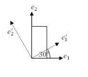
 - The shown rectangle has a length of 2 units and height of 4 units. Find the coordinates of its vertices in the orthonormal basis set
 . Find the coordinates of the vertices in the coordinate system defined by the basis set
  .
.
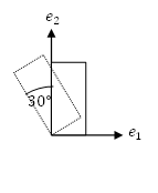
- The shown rectangle has a length of 2 units and height of 4 units. Find the coordinates of its vertices if the rectangle is rotated counterclockwise by the angle shown in the figure. Comment on the difference between the linear mapping used in this problem and that used in the previous problem.
- Verify that the following matrix is an orthogonal matrix, and specify whether it is a rotation or a reflection.
![\[ Q=\left(\begin{matrix}\frac{3}{4}&-\frac{\sqrt{3}}{4}&\frac{1}{2}\\\frac{3\sqrt{3}}{8}&\frac{5}{8}&-\frac{\sqrt{3}}{4}\\-\frac{1}{8}&\frac{3\sqrt{3}}{8}&\frac{3}{4}\end{matrix}\right) \]](https://engcourses-uofa.ca/wp-content/ql-cache/quicklatex.com-7897ec0eb210fe421c3ae8241c9cc534_l3.png "Rendered by QuickLaTeX.com")
- Find the components
 , and
, and  so that the following is a rotation matrix:
![\[Q=\left(\begin{matrix}Q_{11}&Q_{12}&Q_{13}\\\frac{3}{8}+\frac{\sqrt{3}}{4}&\frac{3}{4}-\frac{\sqrt{3}}{8}&-\frac{1}{4}\\\frac{1}{4}-\frac{3\sqrt{3}}{8}&\frac{3}{8}+\frac{\sqrt{3}}{4}&\frac{\sqrt{3}}{4}\end{matrix}\right) \]](https://engcourses-uofa.ca/wp-content/ql-cache/quicklatex.com-8ae7ade3de456224ab417eb128325a04_l3.png "Rendered by QuickLaTeX.com")
- Find the components , and so that the following is a reflection matrix:
![\[Q=\left(\begin{matrix}Q_{11}&Q_{12}&Q_{13}\\\frac{3}{8}+\frac{\sqrt{3}}{4}&\frac{3}{4}-\frac{\sqrt{3}}{8}&-\frac{1}{4}\\\frac{1}{4}-\frac{3\sqrt{3}}{8}&\frac{3}{8}+\frac{\sqrt{3}}{4}&\frac{\sqrt{3}}{4}\end{matrix}\right)\]](https://engcourses-uofa.ca/wp-content/ql-cache/quicklatex.com-58d8883348b2c4f2e2c7d3cf52b0c98e_l3.png "Rendered by QuickLaTeX.com")
- Find two possible combinations for the missing components in so that it is a rotation matrix:
![\[Q=\left(\begin{matrix}0.1&0.2&Q_{13}\\0.1&Q_{22}&Q_{23}\\Q_{31}&Q_{32}&Q_{33}\end{matrix}\right) \]](https://engcourses-uofa.ca/wp-content/ql-cache/quicklatex.com-04fec6535c46af2c97be1c5cece7d81d_l3.png "Rendered by QuickLaTeX.com")
- Find two possible combinations for the missing components in so that it is an orthogonal matrix associated with reflection:
![\[ Q=\left(\begin{matrix}0.1&0.2&Q_{13}\\0.1&Q_{22}&Q_{23}\\Q_{31}&Q_{32}&Q_{33}\end{matrix}\right) \]](https://engcourses-uofa.ca/wp-content/ql-cache/quicklatex.com-5c95da96d1d257d2c924d695b8bd687a_l3.png "Rendered by QuickLaTeX.com")
-
Consider the orthonormal basis set
 and the matrix :
![\[ M=\left(\begin{matrix}1&5&-2\\2&2&3\\-5&2&1\end{matrix}\right) \]](https://engcourses-uofa.ca/wp-content/ql-cache/quicklatex.com-3557766bbea38ab3ca8a531cc68570d3_l3.png "Rendered by QuickLaTeX.com")
- Let
 . Verify that
  and find the vector
  that is orthogonal to both
  , and
, and  . Find a new orthonormal basis set using the normalized vectors of
  , and .
 - Find the components of the matrix in the new orthonormal basis set .
- Find the three invariants of and and verify that they are equal.
- Find the eigenvalues of and and verify that they are equal.
- Find the components of the eigenvectors of and the eigenvectors of and comment on whether they are the same vectors or not.
- Let
- Repeat the previous question with
 , and:
![\[ M=\left(\begin{matrix}-2&5&1\\3&2&2\\1&2&-5\end{matrix}\right) \]](https://engcourses-uofa.ca/wp-content/ql-cache/quicklatex.com-6110096a0b7051048d520cb5a69d4af7_l3.png "Rendered by QuickLaTeX.com")
- Consider the orthonormal basis set and the matrix :
If the orthonormal basis set![\[ M=\left(\begin{matrix}3&0&0\\0&2&1\\0&0&4\end{matrix}\right) \]](https://engcourses-uofa.ca/wp-content/ql-cache/quicklatex.com-bc7e2e90033a41a54e06bc4211878058_l3.png "Rendered by QuickLaTeX.com")
 is used as the coordinate system, find the components of in the new coordinate system.
- Consider the symmetric matrix
 :
:
![\[ S=\left(\begin{matrix}1&0&-2\\0&2&0\\-2&0&1\end{matrix}\right) \]](https://engcourses-uofa.ca/wp-content/ql-cache/quicklatex.com-c8efb94295a6904e4f04045bec5a32ba_l3.png "Rendered by QuickLaTeX.com")
- Find the eigenvalues and eigenvectors of .
- Find a new coordinate system such that the matrix of components
 in the new coordinate system is a diagonal matrix.
- Find the eigenvalues and eigenvectors of
- Identify the positive definite and semi-positive definite symmetric matrices in the following:
![\[ \left(\begin{matrix}1&0&-2\\0&2&0\\-2&0&1\end{matrix}\right)\qquad \left(\begin{matrix}1&0&2\\0&2&0\\2&0&1\end{matrix}\right) \qquad \left(\begin{matrix}1&0&-2\\0&2&0\\-2&0&0\end{matrix}\right)\qquad \left(\begin{matrix}-1&0&-2\\0&2&0\\-2&0&1\end{matrix}\right) \]](https://engcourses-uofa.ca/wp-content/ql-cache/quicklatex.com-07466c4e7d7e0208e454eaf8e8f49343_l3.png "Rendered by QuickLaTeX.com")
- Find the missing values in the components of the orthogonal matrix so that it represents a change of basis while maintaining the proper orientation.
Then, find the components of the identity matrix when a coordinate transformation using![\[ \left(\begin{matrix}\frac{1}{\sqrt{3}}&\frac{1}{\sqrt{3}}&\frac{1}{\sqrt{3}}\\?&?&?\\0&?&\frac{1}{\sqrt{2}}\end{matrix}\right) \]](https://engcourses-uofa.ca/wp-content/ql-cache/quicklatex.com-5ca8bfc135bfebd5b28de874efc1705e_l3.png "Rendered by QuickLaTeX.com") is applied. Comment on the results.
is applied. Comment on the results. - Find the eigenvalues and eigenvectors of the following symmetric matrices and then perform the diagonalization process for each.
![\[ \left(\begin{matrix}11&4&0\\4&5&0\\0&0&7\end{matrix}\right)\qquad \left(\begin{matrix}7&0&-2\\0&5&0\\-2&0&4\end{matrix}\right) \]](https://engcourses-uofa.ca/wp-content/ql-cache/quicklatex.com-db66c7ebb7d828d1509a1ab14ed57948_l3.png "Rendered by QuickLaTeX.com")
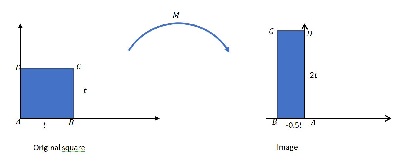
- The figure below shows a square with dimension
 . Determine the transformation matrix
  applied to the object to produce the image shown.
- Let , and
 be three vectors that are linearly independent. Using the properties of the dot product, construct an orthonormal basis set as a function of , and . (The construction is referred to as: Gram-Schmidt Process)
 - Let
 . Find an example of a matrix such that
  . Then, show that if
  is a rotation matrix, then
  .
. - Using Einstein summation convention, and assuming that the underlying space is the Euclidean space
 , show that the following relations hold true for the Kronecker Delta
  and the alternator
  :
:
- Write the following expressions out in full assuming that the underlying space is the Euclidean space :
- Write the following expressions in a compact form using index notation and the Einstein summation convention:
-
![\[ \begin{split}c_{11}x_1+c_{12}x_2+c_{13}x_3 & =d_1\\c_{21}x_1+c_{22}x_2+c_{23}x_3&=d_2 \\ c_{31}x_1+c_{32}x_2+c_{33}x_3&=d_3\end{split} \]](https://engcourses-uofa.ca/wp-content/ql-cache/quicklatex.com-5df89d4ff36ea301896e1ee2eeb34b9d_l3.png "Rendered by QuickLaTeX.com")
 .
.- In the following expressions assume that

![\[\begin{split} \sigma_{11}&=2\mu\varepsilon_{11}+\lambda\varepsilon\\ \sigma_{22}&=2\mu\varepsilon_{22}+\lambda\varepsilon\\ \sigma_{33}&=2\mu\varepsilon_{33}+\lambda\varepsilon\\ \sigma_{12}=\sigma_{21}&=2\mu\varepsilon_{12}=2\mu\varepsilon_{21}\\ \sigma_{13}=\sigma_{31}&=2\mu\varepsilon_{13}=2\mu\varepsilon_{31}\\ \sigma_{32}=\sigma_{23}&=2\mu\varepsilon_{23}=2\mu\varepsilon_{32} \end{split}\]](https://engcourses-uofa.ca/wp-content/ql-cache/quicklatex.com-452e7ead50a2095225412b6badc39794_l3.png "Rendered by QuickLaTeX.com")
-
- Show that symmetric and antisymmetric matrices stay symmetric and antisymmetric, respectively, under any orthogonal coordinate transformation.
- Using the definitions of symmetric and antisymmetric tensors without reference to components.
- Using the component forms of symmetric and antisymmetric matrices.
- In a three dimensional Euclidean vector space, how many independent components will the following tensors have:
- A “completely symmetric” third order tensor.
- A “completely symmetric” fourth order tensor.
 is a completely symmetric fourth order tensor, then:
  .
.
- Show that if
 and
and  are symmetric matrices, then
  is not necessarily a symmetric matrix. (Hint: Find a counter example). On the other hand, show that if and are symmetric matrices that have the same eigenvectors (also called “coaxial”), then and
  are symmetric.
 - Show that if
 is a symmetric matrix, then
  , the matrix
  is symmetric.
 - Let
 and
and  is the identity matrix. Using the algebraic structure of matrices, show that if
  and
and  , then
  . The matrix is referred to as the inverse of and is denoted
  .
. - Let
 be a symmetric matrix. Let
  and
and  be the minimum and maximum eigenvalues of . Show that
  . (The quantity
  is referred to as the Rayleigh Quotient)
 - Let
 . Let be an invertible symmetric matrix. Show the following:


 is symmetric.
- Let be a symmetric matrix. Let
 be another matrix. Find the restriction on to ensure that the matrix
  is symmetric, i.e., that
  . (Hint: in a coordinate system of the eigenvectors of the ratios between the off diagonal components of is equal to the ratios between the corresponding eigenvalues of )
 -
As will be discussed later, the stress at a point can be described as a symmetric matrix with the following form:
Assume a change of coordinates described by the following rotation matrix![\[ \sigma=\begin{pmatrix}\sigma_{11}&\sigma_{12}&\sigma_{13}\\\sigma_{12}&\sigma_{22}&\sigma_{23}\\\sigma_{13}&\sigma_{23}&\sigma_{33}\end{pmatrix} \]](https://engcourses-uofa.ca/wp-content/ql-cache/quicklatex.com-0e21b789bad9ff763a907b7a6b338b82_l3.png "Rendered by QuickLaTeX.com")
In the new coordinate system, the comonents of![\[Q=\begin{pmatrix}\cos{(\theta)}&\sin{(\theta)}&0\\-\sin{(\theta)}&\cos{(\theta)}&0\\0&0&1\end{pmatrix} \]](https://engcourses-uofa.ca/wp-content/ql-cache/quicklatex.com-d4f79e5c4a72a30b2d23d0e97d1eb901_l3.png "Rendered by QuickLaTeX.com")
 will have the following form:
If a vector representation of the stress is adopted as follows:![\[\sigma=Q \sigma Q^T\]](https://engcourses-uofa.ca/wp-content/ql-cache/quicklatex.com-7a2cc24dd1c0274823cbc1beeb3338ba_l3.png "Rendered by QuickLaTeX.com")
Then, show that the components of the vector after transformation are given by:![\[ \sigma_v=\begin{pmatrix}\sigma_{11}\\\sigma_{22}\\\sigma_{33}\\\sigma_{12}\\\sigma_{13}\\\sigma_{23}\end{pmatrix} \]](https://engcourses-uofa.ca/wp-content/ql-cache/quicklatex.com-ec40c9daa7a75e7c26df47a3b79cba9e_l3.png "Rendered by QuickLaTeX.com")
where![\[\sigma_v'=Q_v \sigma_v\]](https://engcourses-uofa.ca/wp-content/ql-cache/quicklatex.com-da7fcb152c08895605b177fb988c3418_l3.png "Rendered by QuickLaTeX.com")
 has the following form:
![\[ Q_v= \left( \begin{array}{cccccc} \cos ^2(\theta) & \sin ^2(\theta) & 0 & \sin (2 \theta) & 0 & 0 \\ \sin ^2(\theta) & \cos ^2(\theta) & 0 & -\sin (2 \theta) & 0 & 0 \\ 0 & 0 & 1 & 0 & 0 & 0 \\ -\frac{1}{2} \sin (2 \theta) & \frac{1}{2} \sin (2 \theta) & 0 & \cos (2 \theta) & 0 & 0 \\ 0 & 0 & 0 & 0 & \cos (\theta) & \sin (\theta) \\ 0 & 0 & 0 & 0 & -\sin (\theta) & \cos (\theta) \\ \end{array} \right) \]](https://engcourses-uofa.ca/wp-content/ql-cache/quicklatex.com-cf0797cdd091134f545a18449efcaf17_l3.png "Rendered by QuickLaTeX.com")


