
Single Degree of Freedom Systems: Undamped Single Degree of Freedom System
A single degree of freedom (SDOF) system is one for which only a single coordinate is required to completely specify the configuration of the system. (This is a suitable working definition for now.) There are typically many possible choices for the coordinate to be used, although some are more natural than others. With a single degree of freedom system, we get one governing differential equation of motion. The specifics of the equation depend on the exact nature of the problem.
We begin our study of vibrations by considering free vibrations of a system. These are the easiest to deal with and understanding these systems is fundamental to understanding more advanced topics in vibration. To keep things as simple as possible, we begin studying undamped free vibrations. The effects of damping will be added in subsequent sections.
Typically in a free vibration problem we have a mass which is displaced from its equilibrium position and then released either from rest or with some initial velocity. Due to the restoring forces in the system, the mass will tend to move back to its equilibrium position but due to its own inertia it will overshoot the equilibrium postion. At some instant the mass will stop momentarily and start to return again to the equilibrium position, and the process will repeat itself (indefinitely if there is no damping). Our goal here is to determine and understand the mathematics used to describe this motion.
Undamped Single Degree of Freedom Systems
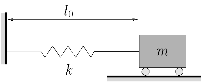
Consider the system shown in Figure 2.1 which is probably the simplest possible vibratory system. Here a body of mass  is attached to a rigid support by a spring with constant stiffness
  . The spring has an unstretched length
  . This is a SDOF system since we need only one coordinate (location of the mass) to completely specify the configuration of the system. There are many possible coordinates we could choose.
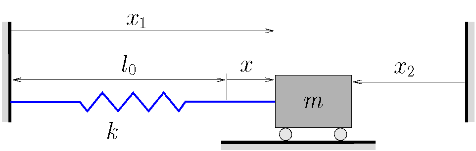
Figure 2.2 shows three possible coordinates, however obviously many others could be chosen as well. In this figure  is measured from the equilibrium position while
  and
and  are measured from other fixed locations. While all of these are valid choices for the coordinate, we will see from our study of vibrations that there are advantages to measuring displacements from the equilibrium position, and so we will chose to do so here.
To obtain the equation of motion we will use Newton’s Laws. To do so we consider the system when it is displaced in the positive coordinate direction and draw a FBD/MAD of the system in this configuration. We additionally assume that the velocity and acceleration of the system are also positive (i.e. in the positive coordinate direction) at this instant. By following this procedure, the signs of all of the terms in our governing equations will be correct and consistent. Note that the positive coordinate direction is determined by the choice of coordinate. In Figure 2.2, the positive direction for and is to the right while for it would be to the left. Any one of these is fine and will work, but once you have decided on your coordinate (and therefore the positive coordinate direction), you must stick with that choice in all that follows.
 as the coordinate (assuming
  )
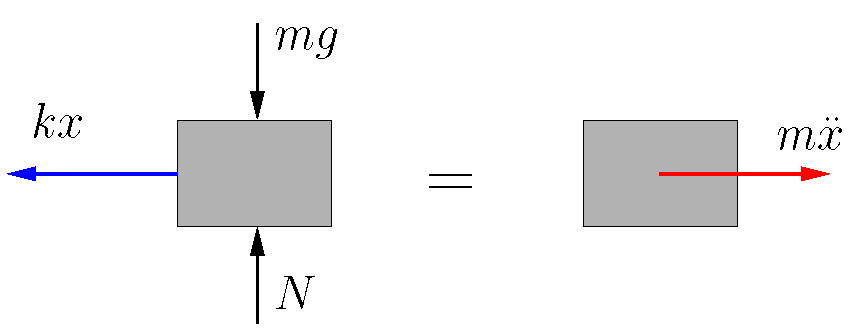
)Figure 2.3 shows the FBD/MAD for our system using as the coordinate. Applying Newton’s Laws we get:
![\[\hspace*{-5cm}\xrightarrow{+}\sum F = ma:\qquad -kx = m \ddot{x}\]](https://engcourses-uofa.ca/wp-content/ql-cache/quicklatex.com-760840403f1d20671048ab2cd6ad8e9a_l3.png "Rendered by QuickLaTeX.com")
or
(2.1) 
Dividing by
results in: ![\[\ddot{x} +\frac{k}{m}x=0\]](https://engcourses-uofa.ca/wp-content/ql-cache/quicklatex.com-5980357766b5de83866c7c42ea2b5fc0_l3.png "Rendered by QuickLaTeX.com")
and defining
(2.2) 
allows equation 2.1 to be written as
(2.3) 
Equation 2.3 is the standard form of the equation of motion for the undamped free vibrations of SDOF system. If a different coordinate had been used it would simply replace in equation 2.3. For example if we had chosen as the coordinate, the equation of motion would have the form
![\[\ddot{x_2}+p^2x_2=0\]](https://engcourses-uofa.ca/wp-content/ql-cache/quicklatex.com-7ea45fff5758463d2679e7c288dd1dcf_l3.png "Rendered by QuickLaTeX.com")
EXAMPLE
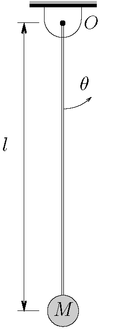
Determine the equation of motion for a simple pendulum of length  and mass
  as shown below. Use
  as the coordinate and assume that only small motions occur.

EXAMPLE
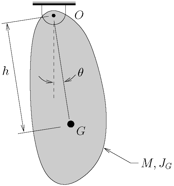
The compound pendulum shown below has a mass and centroidal moment of inertia  . The distance from the support to the center of mass is
  . Determine the equation of motion for this pendulum. Use as the coordinate and assume that only small motions occur.
Solution of Equation 2.3
Equation 2.3 is a second order linear ordinary differential equation (ODE) with constant coefficients. Accordingly, we assume a soltuion of the form:
(2.4) 
which when substituted into Equation 2.3 results in
![\[\left[ \cancel{C} s^2 \cancel{e^{st}} \right] + p^2 \left[ \cancel{C e^{st}} \right] = 0\]](https://engcourses-uofa.ca/wp-content/ql-cache/quicklatex.com-32e4a0e4082ed62839925c87bc06fafd_l3.png "Rendered by QuickLaTeX.com")
or
![\[s^2 + p^2 = 0\]](https://engcourses-uofa.ca/wp-content/ql-cache/quicklatex.com-c5ea56464e855b52d18b8694938fd94f_l3.png "Rendered by QuickLaTeX.com")
which has two roots given by
![\[s = \pm i p\]](https://engcourses-uofa.ca/wp-content/ql-cache/quicklatex.com-ff457b93047211620ac4c79f926b7ac6_l3.png "Rendered by QuickLaTeX.com")
As a result the solution to equation 2.3 becomes
(2.5) 
(Note that  and
and  must be allowed to be complex numbers here.) To proceed we make use of Euler’s identity
![\[\begin{split}e^{ i p t} =&\ \cos{pt}+ i \sin{pt} \\e^{-i p t} =&\ \cos{pt} - i \sin{pt}\end{split}\]](https://engcourses-uofa.ca/wp-content/ql-cache/quicklatex.com-0b78c3ac03350e0cf18090bda77f4ed7_l3.png "Rendered by QuickLaTeX.com")
to write
![\[\begin{split}x(t) =&\ C_1 \bigl[ \cos{pt} + i \sin{pt} \bigr] +C_2 \bigl[ \cos{pt} - i \sin{pt} \bigr] \\[2mm]=&\ \bigl[C_1 + C_2 \bigr] \cos{pt} + \bigl[C_1 - C_2 \bigr] \, i \, \sin{pt}\end{split}\]](https://engcourses-uofa.ca/wp-content/ql-cache/quicklatex.com-35fd2918a3f59668e7bd662fc2b3ce55_l3.png "Rendered by QuickLaTeX.com")
Defining*
![\[\begin{split}A =&\ \bigl[C_1 - C_2 \bigr] \, i \\B =&\ \bigl[C_1 + C_2 \bigr]\end{split}\]](https://engcourses-uofa.ca/wp-content/ql-cache/quicklatex.com-e5093d5c1187aa5ea6e3f657726f5df0_l3.png "Rendered by QuickLaTeX.com")
the solution in equation 2.5 can be written as
(2.6) 
* Note: Since the response of the system in equation 2.6 must be real,  and
and  must be real which implies that and are complex conjugates.
Equation 2.6 is the general solution to equation 2.3 and is the free undamped vibration response of a SDOF system. The response is simple harmonic motion which occurs at a frequency  which is called the natural frequency of the system. For the simple spring mass system we are considering, we see from equation 2.2 that
![\[p = \sqrt{\frac{k}{m}}\]](https://engcourses-uofa.ca/wp-content/ql-cache/quicklatex.com-4bf042977b7e7df2f9f078af8238ef23_l3.png "Rendered by QuickLaTeX.com")
For a general SDOF system, recall that the standard form of the equation of motion is
![\[\ddot{x} + p^2\,x = 0\]](https://engcourses-uofa.ca/wp-content/ql-cache/quicklatex.com-40dd0c6c99bbd85cc1d109a320524261_l3.png "Rendered by QuickLaTeX.com")
The natural frequency, which is a fundamental property of a vibrating system, can be determined by inspection if the equation of motion is expressed in this standard form. Note that in equation 2.3 is always in units of rad/s.
There are two unknown constants and in equation 2.6. We determine their values typically by considering the initial conditions for the system. Since we have a two unknown constants, we need to specify two initial conditions. These are typically the starting position and velocity of the mass. For example, at a start time  we could have
![\[\begin{split}x(0) &= x_0 \\\dot{x}(0) &= v_0\end{split}\]](https://engcourses-uofa.ca/wp-content/ql-cache/quicklatex.com-9f105ac51b004f150a13c89d0bf174eb_l3.png "Rendered by QuickLaTeX.com")
(where
 or
or  could be negative). Equation 2.6 then gives
![\[x(0) = x_0 = A \, \cancelto{0}{\sin\left({p\cdot 0}\right)} + B \, \cancelto{1}{\cos\left({p\cdot 0}\right)}\]](https://engcourses-uofa.ca/wp-content/ql-cache/quicklatex.com-c64ec583e30bf04eef48dba7992d261f_l3.png "Rendered by QuickLaTeX.com")
so that
![\[B = x_0\]](https://engcourses-uofa.ca/wp-content/ql-cache/quicklatex.com-c370e20607025831ab4032b757dd4cf6_l3.png "Rendered by QuickLaTeX.com")
Differentiating equation 2.6
![\[\dot{x} = A p \cos{pt} - B p \sin{pt}\]](https://engcourses-uofa.ca/wp-content/ql-cache/quicklatex.com-3af9b7df5f919bca0a5ad27750316de0_l3.png "Rendered by QuickLaTeX.com")
and using the second initial condition leads to
![\[\dot{x}(0) = v_0 = A p \, \cancelto{1}{\cos\left({p\cdot 0}\right)} -B p \, \cancelto{0}{\sin\left({p\cdot 0}\right)}\]](https://engcourses-uofa.ca/wp-content/ql-cache/quicklatex.com-73d331d1796a5ba132d41bf0dd13bd78_l3.png "Rendered by QuickLaTeX.com")
or
![\[A = \frac{v_0}{p}\]](https://engcourses-uofa.ca/wp-content/ql-cache/quicklatex.com-09f07371a75f8e56c00730188b4ad9ee_l3.png "Rendered by QuickLaTeX.com")
The response of the system is therefore given by
(2.7) 
which completely specifies the response of the system for all time
 .
.
Other forms of the General response
While equation 2.7 represents the response of the SDOF undamped system, the solution may be expressed in other equivalent forms:

where
![\[\begin{split}\mathbb{X} &= \sqrt{x_0^2 + \left(\frac{v_0}{p}\right)^2} \\\phi &= \tan^{-1}\biggl[ \frac{x_0}{v_0/p} \biggr]\end{split}\]](https://engcourses-uofa.ca/wp-content/ql-cache/quicklatex.com-62fa72feaf9e4392712a7a97d1005323_l3.png "Rendered by QuickLaTeX.com")

where
![\[\begin{split}\mathbb{X} &= \sqrt{x_0^2 + \left(\frac{v_0}{p}\right)^2}\\\alpha &= \tan^{-1}\biggl[ \frac{v_0/p}{x_0} \biggr]\end{split}\]](https://engcourses-uofa.ca/wp-content/ql-cache/quicklatex.com-dd3c787ebb6d37c6868434ced24d0054_l3.png "Rendered by QuickLaTeX.com")
These relationships are shown in Figure 2.4. Note that 
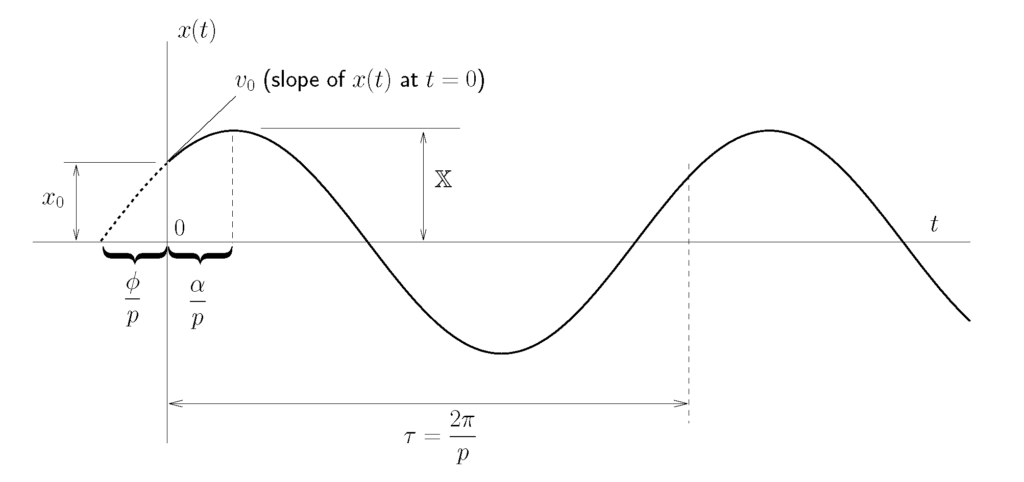
Period and Frequency
The period  is the time required for the harmonic motion to repeat itself (i.e. to complete one cycle). is related to the natural frequency by
(2.8) 
so that
![\[\tau = \frac{2 \pi}{p} \qquad\text{or}\qquad p = \frac{2 \pi}{\tau}\]](https://engcourses-uofa.ca/wp-content/ql-cache/quicklatex.com-18da3bada10366f32ced7517199e519f_l3.png "Rendered by QuickLaTeX.com")
Another common unit for frequency measurement is Hertz (Hz) or cycles per second. Since there are  radians per complete cycle, we note that
(2.9) 
where  is the natural frequency expressed in Hertz. Similar to Equation 2.8 we note that
![\[\boxed{f_n \cdot \tau = 1}\]](https://engcourses-uofa.ca/wp-content/ql-cache/quicklatex.com-f52859d8179086325d608239beace538_l3.png "Rendered by QuickLaTeX.com")
Rotating Vector Representation
We can also think of the response of the undamped SDOF system in terms of rotating vectors (another way of thinking about a subject is often helpful). Consider two vectors, with magnitudes and , fixed  apart rotating CCW with an angular velocity as shown in Figure 2.5.
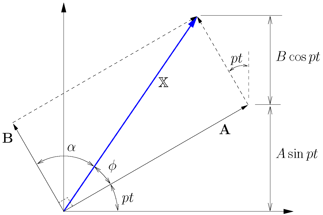
The (vector) sum of  and
and  is another vector
  with a magnitude
![\[\mathbb{X} = \sqrt{A^2 + B^2}\]](https://engcourses-uofa.ca/wp-content/ql-cache/quicklatex.com-743e22313bf341a8a15fb4ca520f04b0_l3.png "Rendered by QuickLaTeX.com")
which also rotates at a rate
. The fixed angles  and
and  can be seen to be
![\[\begin{split}\phi &= \tan^{-1} \biggl[ \frac{B}{A} \biggr] \\\alpha &= \tan^{-1} \biggl[ \frac{A}{B} \biggr]\end{split}\]](https://engcourses-uofa.ca/wp-content/ql-cache/quicklatex.com-52bf81869ce2ecf7f6308e2b24500510_l3.png "Rendered by QuickLaTeX.com")
Now, guided by our previous results
![\[x(t) = \frac{v_0}{p} \sin{pt} + x_0 \cos{pt}\]](https://engcourses-uofa.ca/wp-content/ql-cache/quicklatex.com-d8fd37f48c799473013be1885d91b259_l3.png "Rendered by QuickLaTeX.com")
we see that if we let
![\[\begin{split}A &= \frac{v_0}{p}, \\B &= x_0,\end{split}\]](https://engcourses-uofa.ca/wp-content/ql-cache/quicklatex.com-e0c6b21842b5143d15ca1935d7fba325_l3.png "Rendered by QuickLaTeX.com")
then the position  can be interpreted as the vertical component of the rotating vector . As can be seen from Figure 2.5, this vertical component can be expressed as
![\[\begin{split}x(t) &= \frac{v_0}{p} \sin{pt}+ x_0 \cos{pt} \\&= \mathbb{X} \sin{(pt+\phi)}\\\intertext{or}&= \mathbb{X} \cos\bigl(p t - \alpha\bigr)\end{split}\]](https://engcourses-uofa.ca/wp-content/ql-cache/quicklatex.com-69ca849c2daa31204b79c5e99ac4ef31_l3.png "Rendered by QuickLaTeX.com")
which agrees with our previous results (noting that
 ).
).
Energy Methods
For conservative systems we can also use an energy approach to obtain the equations of motion. Since the total mechanical energy is conserved in these systems, the sum of the kinetic energy  and the potential energy
  will be a constant
(2.10) 
where the actual value of the constant can be evaluated, if necessary, from the initial conditions. Differentiating Equation 2.10 with respect to time gives
![\[\frac{d}{dt}\Bigl(T+U\Bigr) = 0\]](https://engcourses-uofa.ca/wp-content/ql-cache/quicklatex.com-3ee4b6e27aeea3a1f38fa845d835eae9_l3.png "Rendered by QuickLaTeX.com")
which leads directly to the equation of motion for the system.
Consider the simple spring-mass system in Figure 2.1 with configuration described by the coordinate measured from the equilibrium position. The potential energy stored in the spring when the mass is at some location is given by
![\[U = \frac{1}{2} k x^2\]](https://engcourses-uofa.ca/wp-content/ql-cache/quicklatex.com-fd02985632b5b562eb4e66f3c5f3a45b_l3.png "Rendered by QuickLaTeX.com")
Similarly, since  represents the speed of the mass, the kinetic energy in the system is
![\[T= \frac{1}{2} m \dot{x}^2\]](https://engcourses-uofa.ca/wp-content/ql-cache/quicklatex.com-f3e2ff7e4af73bf57da62e2364ff8a4f_l3.png "Rendered by QuickLaTeX.com")
Since this system is conservative, the total mechanical energy can be expressed as
![\[\frac{1}{2} m \dot{x}^2 + \frac{1}{2} k x^2 = \text{constant}\]](https://engcourses-uofa.ca/wp-content/ql-cache/quicklatex.com-e8d9544d5b8036e3e33f79022e5c4ad2_l3.png "Rendered by QuickLaTeX.com")
and differentiating with respect to time yields
![\[\frac{1}{2} m \left(2\dot{x}\right)\ddot{x} +\frac{1}{2} k \left(2 x\right)\dot{x} = 0\]](https://engcourses-uofa.ca/wp-content/ql-cache/quicklatex.com-3342f7dfd1a2f779f808f1da0f692468_l3.png "Rendered by QuickLaTeX.com")
(2.11) 
Equation 2.11 must hold for all times  and for all values of . The only way this can be satisfied (since
  for all times ) is to require that
![\[m \ddot{x} + k x = 0\]](https://engcourses-uofa.ca/wp-content/ql-cache/quicklatex.com-1241566487f55f5f1a82f47abb7024df_l3.png "Rendered by QuickLaTeX.com")
at all times which is the equation of motion for the system obtained previously.
Note that if we have a conservative system and we assume harmonic motion at the start, we can obtain the natural frequency somewhat more directly. For such a system, the mechanical energy is continually converted between potential and kinetic energy. At the extremes of the motion, when the mass momentarily stops and changes direction, there is no kinetic energy in the system so that all of the energy is potential energy. Hence potential energy is at a maximum value  . Similarly, when the mass is moving past the equilibrium position, the potential energy is a minimum while the kinetic energy has a maximum value
  . If we make the assumption that the potential energy of the system is zero at the equilibrium position, then these two maximum values for the energy will have the same value, i.e.
(2.12) 
Again, consider the simple spring-mass system (with coordinate measured from the equilibrium position). If we assume the system undergoes simple harmonic motion given by
![\[x(t) = \mathbb{X} \sin{(pt+\phi)}\]](https://engcourses-uofa.ca/wp-content/ql-cache/quicklatex.com-6dec8432b802766ff9fcf806cb9659ed_l3.png "Rendered by QuickLaTeX.com")
then the maximum displacement is so that
![\[U_{max} = \frac{1}{2} k \mathbb{X}^2\]](https://engcourses-uofa.ca/wp-content/ql-cache/quicklatex.com-2c6c6db956d5163841ef129941f281ac_l3.png "Rendered by QuickLaTeX.com")
Similarly, the speed is given by
![\[\dot{x}(t) = p\mathbb{X} \cos{(pt+\phi)}\]](https://engcourses-uofa.ca/wp-content/ql-cache/quicklatex.com-dc056068cd282219d5c177bdb790524c_l3.png "Rendered by QuickLaTeX.com")
which has a maximum value of  so that
![\[T_{max} = \frac{1}{2} m \bigl(p \mathbb{X}\bigr)^2\]](https://engcourses-uofa.ca/wp-content/ql-cache/quicklatex.com-698577419f3cd82db116ee181bdb426f_l3.png "Rendered by QuickLaTeX.com")
Substituting these expressions into Equation 2.12 gives
![\[\frac{1}{2} m \bigl(p \mathbb{X}\bigr)^2 = \frac{1}{2} k \mathbb{X}^2\]](https://engcourses-uofa.ca/wp-content/ql-cache/quicklatex.com-cf59128887749231da9469a52a04d42f_l3.png "Rendered by QuickLaTeX.com")
which can be solved for as
which is the natural frequency of the system found previously.
This approach is known as Rayleigh’s Method and we will encounter variations of this approach later on in the course. Note that this approach is limited to conservative systems which have zero potential energy at the equilibrium position.
EXAMPLE
Using an energy approach, determine the equation of motion for a simple pendulum of length and mass as shown below. Use as the coordinate and assume that only small motions occur.
I have a task. The given equation is same as equation 2.1, initial velocity is 1m/s and displacement is 1m. How to find out the displacement and velocity during the first 5 seconds?