Engineering at Alberta Courses » Application to Lateral Vibrations of Beams

Approximate Methods for Continuous Systems: Application to Lateral Vibrations of Beams

The systems we have considered so far have been relatively simple so we were able to find analytical solutions. This is usually possible in only the simplest situations. For more complicated systems, say ones which include

non-uniform material properties and/or cross sections, or
more complicated boundary conditions,

it is very difficult, if not impossible, to determine analytical solutions. In these situations we usually resort to numerical solutions. Sometimes however, other approximate techniques can also be useful. In particular, Rayleigh’s Method is well suited for use with continuous systems.

Recall that for discrete systems, Rayleigh’s Quotient was expressed as

(11.1) $\begin{equation*} p^2 = \frac { \{\Phi\}^T \text{[}k\text{]} \{\Phi\}} { \{\Phi\}^T \text{[}m\text{]} \{\Phi\} } \end{equation*}$

where $\text{[}k\text{]}$ is the stiffness matrix, $\text{[}m\text{]}$ is the mass matrix and { $\Phi$ } is a mode shape vector. To determine an approximate natural frequency, a trial mode shape vector { $\Phi$ } is used in 11.1 to return an upper limit on the lowest natural frequency.

To apply Rayleigh’s Quotient to continuous systems, we recall that Rayleigh’s Quotient is based on the idea that the maximum kinetic energy and the maximum potential energy in a conservative system will be equal. This requires that the potential energy be zero in the equilibrium configuration.

$\begin{equation*} T_{MAX} = U_{MAX} \end{equation*}$

when all of the masses in the system undergo simple simultaneous harmonic motion, as happens in the modal responses.

We can also apply this idea to continuous systems. If $u(x,t)$ is some representative displacement function, the procedure will be to

Estimate the fundamental mode shape $U(x)$ .
Assume simple simultaneous harmonic motion of the form $u(x,t) = U(x))\sin{(pt +\phi)}$
Determine the maximum potential energy $U_{MAX}$ .
Determine the maximum kinetic energy $T_{MAX}$
Set $U_{MAX} = T_{MAX}$ and solve for $p$

It is important here that the mode shape assumed in step (a) satisfies the (geometric) boundary conditions of the problem. If this is the case then the frequency $p$ determined by this procedure will again be an upper bound on the lowest natural frequency. If the assumed mode shape doesn’t satisfy the (geometric) boundary conditions in the problem, then we no longer have this guarantee.

To apply Rayleigh’s Method to beams, we need to be able to determine the potential and kinetic energies associated with a beam vibrating in a given assumed mode shape.

Potential Energy

Potential energy is stored in a beam as elastic (strain) energy. In most cases the energy stored due to bending is much larger than that stored due to shear or axial forces. As a result only the energy associated with bending is usually considered.

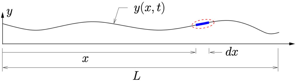
(a) Deformed Body

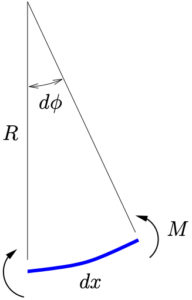
(b) Infinitesimal Element
Figure 11.1: Initially straight beam in arbitrary deformed configuration

Consider an initially straight beam, deformed to some arbitrary configuration $y(x,t)$ (limited to small motions) during its motion as shown in Figure 11.1{a}. Figure 11.1{b} shows an infinitesimal element of the beam during this motion. At this point the beam element has a radius of curvature~ $R$ which is related to the included angle $d\phi$ by

(11.2) $\begin{equation*} d\phi = \frac{dx}{R}. \end{equation*}$

For an elastic beam the bending moment is related to the deflection (curvature) by

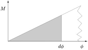
(11.3) $\begin{equation*} M = EI\frac{1}{R}. \end{equation*}$

Now, consider the infinitesimal work done on the beam element as it is deformed from its initially unloaded straight (equilibrium) configuration to one with an included angle $d\phi$ as shown in Figure 11.1{b}. The work is

$\begin{equation*} dW = \frac{1}{2} M d\phi \end{equation*}$

which is equal to the area under the $M$ – $\phi$ graph as shown. For an elastic beam, this work done on the beam is equal to the strain energy $dU$ stored in the beam element, so that we get

$\begin{equation*} dU = dW = \frac{1}{2} M d\phi. \end{equation*}$

Using equation 11.2 and equation 11.3 this becomes

$\begin{equation*} dU &= \frac{1}{2} \biggl[ EI\frac{1}{R} \biggr] \biggl[ \frac{dx}{R} \biggr] \end{equation*}$

(11.4) $\begin{align*} dU &= \frac{1}{2} EI \biggl( \frac{1}{R} \biggr)\!\!\rule[7mm]{0pt}{0pt}^2 dx. \end{align*}$

For small deflections,

$\begin{equation*} \frac{1}{R} \approx \frac{\partial^2 y}{\partial x^2} \end{equation*}$

so 11.4 becomes

(11.5) $\begin{equation*} dU = \frac{1}{2} EI \biggl( \frac{\partial^2 y}{\partial x^2} \biggr)\!\!\rule[7mm]{0pt}{0pt}^2 dx, \end{equation*}$

which gives the strain energy stored in the infintesimal beam element. To find the total strain energy stored, we integrate over the length of the beam

(11.6) $\begin{align*} U &= \int\limits_{\text{beam}} dU \nonumber \\ &= \frac{1}{2} \int_0^L EI \biggl( \frac{\partial^2 y}{\partial x^2} \biggr)\!\!\rule[7mm]{0pt}{0pt}^2 dx. \end{align*}$

If we make the usual assumption that the motion of the beam is of the form

$\begin{equation*} y(x,t) = Y(x) \sin{(pt +\phi)}, \end{equation*}$

then

$\begin{equation*} \frac{\partial^2 y}{\partial x^2} = \frac{d^2 Y}{dx^2} \sin{(pt +\phi)}, \end{equation*}$

so equation 11.6 becomes

(11.7) $\begin{equation*} U = \frac{1}{2} \int_0^L EI \biggl[ \frac{d^2 Y}{dx^2} \sin{(pt +\phi)} \biggr]^2 dx. \end{equation*}$

The maximum strain energy occurs when

$\begin{equation*} \sin{(pt +\phi)} = \pm 1 \end{equation*}$

which occurs at the same instant for every point on the beam. Using 11.7 we find that

(11.8) $\begin{equation*} \boxed{U_{MAX }= \frac{1}{2} \int_0^L EI \biggl[ \frac{d^2 Y}{dx^2} \biggr]^2 dx.} \end{equation*}$

Equation 11.8 represents the maximum strain energy stored in the beam for a given (assumed) mode shape $\mathbb{Y}(x)$ . Note that since

$\begin{equation*} M = EI \frac{d^2 Y}{dx^2}, \end{equation*}$

Equation 11.8 can equivalently be written as

(11.9) $\begin{equation*} \boxed{U_{MAX} = \frac{1}{2} \int_0^L \biggl[ \frac{M^2(x)}{EI} \biggr] dx,} \end{equation*}$

which may be easier to use in some cases.

Kinetic Energy

Once again consider the infinitesimal beam element shown in Figure 11.1(b). The kinetic energy of that element is given by

$\begin{equation*} dT = \frac{1}{2}\, dm\, v^2 \end{equation*}$

where

$\begin{equation*} dm = \rho A dx \end{equation*}$

is the mass of the infinitesimal element and its speed is given by (This considers only the translational kinetic energy and ignores any rotational energy, i.e. Euler beam theory.)

$\begin{equation*} v = \frac{\partial y}{\partial t}. \end{equation*}$

Assuming once again that the motion of the beam is of the form

$\begin{equation*} y(x,t) = \mathbb{Y}(x) \sin{(pt +\phi)} \end{equation*}$

then

(11.10) $\begin{equation*} \frac{\partial y}{\partial t} = \mathbb{Y}(x) p \cos{(pt + \phi)}. \end{equation*}$

Therefore the kinetic energy becomes

$\begin{equation*} dT = \frac{1}{2} \rho A \biggl[ \mathbb{Y}(x) p \cos{(pt + \phi)} \biggr]^2 dx. \end{equation*}$

The total kinetic energy in the beam is then obtained by integration

$\begin{align*} T &= \int\limits_{\text{beam}} dT \\ &= \frac{1}{2} \, p^2 \int_0^L \! \rho A \biggl[ \mathbb{Y}(x) \cos{(pt + \phi)} \biggr]^2 dx. \end{align*}$

This is a maximum when

$\begin{equation*} \cos{(pt + \phi)} = \pm 1 \end{equation*}$

which occurs simultaneously at all points on the beam. Therefore the maximum kinetic energy in the vibrating beam is

(11.11) $\begin{equation*} \boxed{T_{MAX} = \frac{1}{2} \, p^2 \int_0^L \! \rho A \Bigl[ \mathbb{Y}(x) \Bigr]^2 dx.} \end{equation*}$

Rayleigh’s Quotient For Lateral Vibrations of Beams

As we have seen previously, for a conservative system,

$\begin{equation*} T_{MAX} = U_{MAX}. \end{equation*}$

Using equation 11.8 and equation 11.11 this becomes

$\begin{equation*} {\frac{1}{2}} \, p^2 \int_0^L \rho A \Bigl[ \mathbb{Y}(x) \Bigr]^2 dx = {\frac{1}{2}} \int_0^L EI \biggl[ \frac{d^2 \mathbb{Y}}{dx^2} \biggr]^2 dx \end{equation*}$

(11.12) $\begin{equation*} \boxed{p^2 = \dfrac{\int\limits_0^L EI \biggl[ \dfrac{d^2 \mathbb{Y}}{dx^2} \biggr]^2 dx} {\int\limits_0^L \rho A \Bigl[ \mathbb{Y}(x) \Bigr]^2 dx}.} \end{equation*}$

Equation 11.12 is Rayleigh’s Quotient for beam applications where, as in the multiple degree of freedom cases discussed previously, $\mathbb{Y}(x)$ is an assumed mode shape for the beam. If the assumed mode shape satisfies the geometric boundary conditions in the system, the natural frequency obtained using equation 11.12 will be an upper bound on the lowest (fundamental) natural frequency.

Example

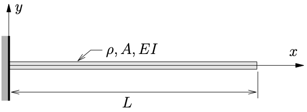
Estimate the fundamental natural frequency of a uniform cantilever beam of length $L$ ( $\rho, A, E, I$ are all constants). Assume a mode shape of
$\begin{equation*} \mathbb{Y}(x) = C x^2. \end{equation*}$
Repeat the calculation in part (1) but instead use an assumed shape function
$\begin{equation*} \mathbb{Y}(x) = \frac{1}{6EI} \Bigl(3 L x^2 - x^3 \Bigr) \end{equation*}$

which is the static equilibrium shape of the beam when it is subjected to a unit tip load. Compare these predictions to the true fundamental natural frequency

$\begin{equation*} p_1 \approx 3.516 \sqrt{\frac{EI}{\rho A L^4}}. \end{equation*}$

Extensions to Rayleigh’s Method for Beams

For beams, Rayleigh’s Quotient, given by 11.12 was obtained by considering the ratio of the maximum potential and kinetic energies in the system. We can extend this idea to consider additional springs and masses in the system.

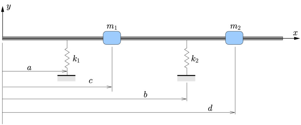
Figure 11.2: Beam with additional masses and supports

Consider the system shown in Figure 11.2. To determine the potential energy stored in the system for an assumed mode shape $\mathbb{Y}(x)$ , we can include the potential energy stored in the springs as additional terms

$\begin{equation*} \frac{1}{2} k_1 \Bigl[ \mathbb{Y}(a) \Bigr]^2 + \frac{1}{2} k_2 \Bigl[ \mathbb{Y}(b) \Bigr]^2 \end{equation*}$

where $\mathbb{Y}(a)$ and $\mathbb{Y}(b)$ are the deflections of the beam at locations $x=a$ and $x=b$ respectively. The maximum potential energy stored in the systems then becomes

(11.13) $\begin{equation*} \boxed{U_{MAX} = \frac{1}{2} \int_0^L EI \biggl[ \dfrac{d^2 \mathbb{Y}}{dx^2} \biggr]^2 dx + \frac{1}{2} k_1 \Bigl[ \mathbb{Y}(a)\Bigr]^2 + \frac{1}{2} k_2 \Bigl[ \mathbb{Y}(b)\Bigr]^2.} \end{equation*}$

Similarly, the extra kinetic energy in the beam due to the additional masses is given by

$\begin{equation*} \frac{1}{2} m_1 v_1^2 + \frac{1}{2} m_2 v_2^2, \end{equation*}$

where

$\begin{equation*} v_1 = \frac{\partial y}{\partial t}\biggr|_{x=c},\qquad v_2 = \frac{\partial y}{\partial t}\biggr|_{x=d}. \end{equation*}$

However, we have seen in equation 11.10 that

$\begin{equation*} \frac{\partial y}{\partial t} = \mathbb{Y}(x) \, p \cos{(pt + \phi)} \end{equation*}$

so that the speeds become

$\begin{align*} v_1 &= \mathbb{Y}(c) \, p \cos{(pt + \phi)}, \\ v_2 &= \mathbb{Y}(d) \, p \cos{(pt + \phi)}. \end{align*}$

These will be maximum when $\cos{(pt + \phi)}=1$ so that the maximum additional kinetic energy is

$\begin{equation*} \frac{1}{2} m_1 p^2 \Bigl[\mathbb{Y}(c)\Bigr]^2 + \frac{1}{2} m_2 p^2 \Bigl[\mathbb{Y}(d)\Bigr]^2. \end{equation*}$

As a result the total maximum kinetic energy in the system is given by

(11.14) $\begin{equation*} \boxed{T_{MAX} = \frac{1}{2} \, p^2 \int_0^L \rho A \Bigl[ \mathbb{Y}(x) \Bigr]^2 dx + \frac{1}{2} m_1 p^2 \Bigl[\mathbb{Y}(c)\Bigr]^2 + \frac{1}{2} m_2 p^2 \Bigl[\mathbb{Y}(d)\Bigr]^2.} \end{equation*}$

Equating 11.13 and equation 11.14 we see that

$\begin{equation*} \begin{split} {\frac{1}{2}} p^2 \int_0^L \rho A \Bigl[ \mathbb{Y}(x) \Bigr]^2 dx + {\frac{1}{2}} m_1 p^2 \Bigl[\mathbb{Y}(c)\Bigr]^2 + {\frac{1}{2}} m_2 p^2 \Bigl[\mathbb{Y}(d)\Bigr]^2 = \\ {\frac{1}{2}} \int_0^L EI \biggl[ \dfrac{d^2 \mathbb{Y}}{dx^2} \biggr]^2 dx + {\frac{1}{2}} k_1 \Bigl[ \mathbb{Y}(a)\Bigr]^2 +{\frac{1}{2}} k_2 \Bigl[ \mathbb{Y}(b)\Bigr]^2 \end{split} \end{equation*}$

$\begin{equation*} p^2 = \dfrac{\int\limits_0^L EI \biggl[ \dfrac{d^2 \mathbb{Y}}{dx^2} \biggr]^2 dx + k_1 \Bigl[ \mathbb{Y}(a)\Bigr]^2 + k_2 \Bigl[ \mathbb{Y}(b)\Bigr]^2} {\int\limits_0^L \rho A \Bigl[ \mathbb{Y}(x) \Bigr]^2 dx + m_1 \Bigl[\mathbb{Y}(c)\Bigr]^2 + m_2 \Bigl[\mathbb{Y}(d)\Bigr]^2}. \end{equation*}$

This can be generalized to a beam with $r$ masses and $s$ springs as

(11.15) $\begin{equation*} \boxed{p^2 = \dfrac{\int\limits_0^L EI \biggl[ \dfrac{d^2 \mathbb{Y}}{dx^2} \biggr]^2 dx + \sum\limits_{i=1}^{s} k_i \Bigl[ \mathbb{Y}(x_i)\Bigr]^2} {\int\limits_0^L \rho A \Bigl[ \mathbb{Y}(x) \Bigr]^2 dx + \sum\limits_{j=1}^{r} m_j \Bigl[ \mathbb{Y}(x_j)\Bigr]^2}.} \end{equation*}$

Example 1

A driveshaft for a marine propeller can be modeled as shown below.

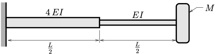
Estimate the fundamental natural frequency using Rayleigh’s quotient. Assume a mode shape of
$\begin{equation*} \mathrm{Y}(x) = C x^3 \end{equation*}$

and neglect the mass of the shaft.
An alternative design for this propeller features a uniform shaft stiffened with an intermediate bearing (with stiffness $k$ ) as shown below.

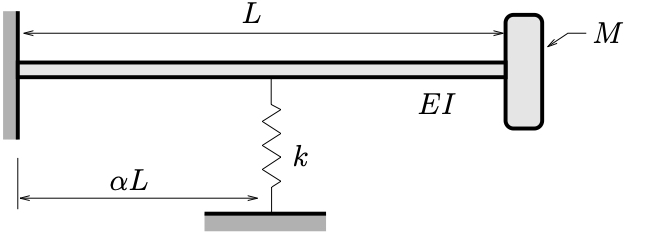Estimate the location $\alpha$ for this bearing such that the natural frequency of the alternate design is the same as for the original design. Express your answer in terms of $EI, L$ and $k$ .
Use the same assumed mode shape $\mathrm{Y}(x) = C x^3$ and once again neglect the mass of the shaft in your calculations.

Example 2

Two views of an airplane wing are shown in which the wing is modeled as a cantilever that has a varying stiffness $EI$ and a wing tank of mass $M$ when filled with aviation gasoline.

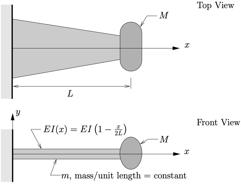
Determine an expression for the lowest natural frequency of free vertical vibrations of the wing and fuel tank. Assume a trial function
$\begin{equation*} Y(x) = D x^2. \end{equation*}$
If the natural frequency is not to be more than 25% greater when the tank is empty ( $M=0$ ) than when it is full (mass $M$ is included), determine the maximum mass $M$ which can be added in comparison to the mass of the wing itself.

Open Educational Resources