Vibrations of Continuous Systems: Transverse Vibrations of a Cable
In the systems considered so far, all of the masses in the system were either particles or rigid bodies so that only a finite number of coordinates were required to specify their configuration. As well, the stiffness and damping elements (springs and dashpots) were generally considered to be massless and act at a single location.
While this approach can serve to model a wide variety of systems reasonably well, there are also other kinds of problems for which such an approach does not give a sufficiently complete understanding. In such systems we may have to consider the mass (and possibly the stiffness and damping) to be distributed throughout the system continuously. These systems are known as distributed or continuous systems as opposed to the discrete or lumped parameter systems that have so far been considered.
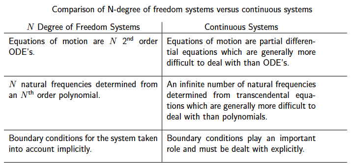
The fundamental difference between these two types of systems is that an infinite number of coordinates are required to completely specify the configuration of a continuous system as opposed to a finite number for the discrete systems we have been considering.
However, many of the fundamental concepts we have developed for \mdof systems are still applicable to continuous systems although as you might expect the math gets more involved.
One of the simplest examples of a continuous vibrating system is the transverse motions of an elastic cable under a tension  . To keep the system as simple as possible we assume that the cable is uniform with a constant linear density
  (mass/unit length). We further assume that the deflections are small. This assumption is required to keep the equations linear and implies, among other things, that the tension in the cable remains approximately constant throughout the motion.
Equations of Motion
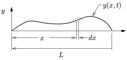
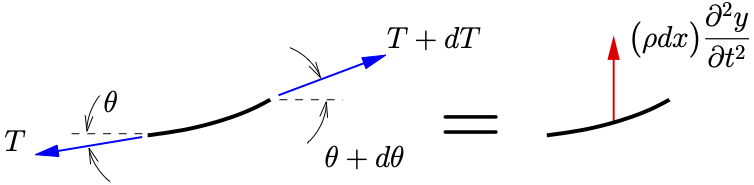
Figure 10.1: Elastic cable undergoing small motions.
Figure 10.1(a) shows a cable of length  , pinned at both ends, in an arbitrary deformed configuration. The deflected shape of the cable is given by
  (Note that we need a function to describe the configuration rather than a vector of a finite number of coordinates). Consider an infinitesimal element of the cable, at position
  , of length
  as indicated. A FBD/MAD of the infinitesimal element is shown in Figure 10.1(b). Applying Newton’s Laws in the horizontal direction we find

For small deflections,  is small so that

and the above becomes

so that
(10.1) 
This shows that the tension in the cable can be considered to be constant (to a first order approximation) as long as the motion of the cable remains small. Now, applying Newton’s Laws in the vertical direction we have
![\[+\!\!\uparrow\sum F = ma:\qquad-T \cancelto{\theta}{\sin(\theta)} + \bigl(T + \cancelto{0}{dT}\bigr) \cancelto{\theta + d\theta}{\sin(\theta} + d\theta) = \rho \, dx \, \frac{\partial^2 y}{\partial t^2}\]](https://engcourses-uofa.ca/wp-content/ql-cache/quicklatex.com-d0faf08cb09a2c04986cd826f50c0921_l3.png "Rendered by QuickLaTeX.com")
where  is the mass of the element. For small motions we can further approximate
  as
as

As a result the equation of motion in the vertical direction becomes
![\begin{align*}-\ensuremath{T} \, \theta + \ensuremath{T} \bigl(\theta + \frac{\partial \theta}{\partial x} dx\bigr)&= \rho \, dx \ensuremath{\frac{\partial^2 y}{\partial t^2}} \\{-\ensuremath{T} \theta + \ensuremath{T} \theta} + \ensuremath{T} \frac{\partial \theta}{\partial x} dx&= \rho \, dx \ensuremath{\frac{\partial^2 y}{\partial t^2}} \\[2mm]\ensuremath{T} \frac{\partial \theta}{\partial x} {dx} &= \rho \, {dx} \ensuremath{\frac{\partial^2 y}{\partial t^2}}\end{align*}](https://engcourses-uofa.ca/wp-content/ql-cache/quicklatex.com-b4a3a9bc1a84790dc906771cfed4545d_l3.png "Rendered by QuickLaTeX.com")
or

However, for small angles,  so that the equation of motion becomes

or finally
(10.2) 
where
(10.3) 
10.2 is a partial differential equation for  and is known as the wave equation. The term
  in 10.3 has units of
  and is known as the wave speed.
Solution to the Wave Equation
When we considered multiple degree of freedom systems, the solutions to the free vibration problem were of the form of a mode shape undergoing simple simultaneous harmonic motion,

Guided by this result, when dealing with continuous systems we will similarly look for solutions of the form of a particular mode shape undergoing motion that is a function of time. We therefore assume that
(10.4) 
where
 is the mode shape which is a function of only, and
 is a function of
  only and represents the time varying nature of the motion.
Note: This approach is formally known as the separation of variables technique.
With this assumption, we find that
![\begin{align*}\ensuremath{\frac{\partial^2 y}{\partial x^2}} &= \frac{d^2 \ensuremath{\mathbb{Y}}}{d x^2} \, \ensuremath{\mathbb{T}}(t) \\[2mm]\ensuremath{\frac{\partial^2 y}{\partial t^2}} &= \ensuremath{\mathbb{Y}}(x) \, \frac{d^2 \ensuremath{\mathbb{T}}}{d t^2}\end{align*}](https://engcourses-uofa.ca/wp-content/ql-cache/quicklatex.com-9a0fa5dbdf7692c65e9ee9071da8de71_l3.png "Rendered by QuickLaTeX.com")
which when substituted into the equation of motion 10.2 gives

or upon rearranging
(10.5) 
Since the LHS and RHS of 10.5 must equal each other at all positions and at all times , the only possible solution is if both sides are equal to a constant. This results in two ordinary differential equations which, letting the constant be  , can be written as
![\begin{align*}\frac{\ensuremath{c}^2}{\ensuremath{\mathbb{Y}}(x)} \frac{d^2 \ensuremath{\mathbb{Y}}}{d x^2} &= -p^2 \\[2mm]\frac{1}{\ensuremath{\mathbb{T}}(t)} \frac{d^2 \ensuremath{\mathbb{T}}}{d t^2} &= -p^2\end{align*}](https://engcourses-uofa.ca/wp-content/ql-cache/quicklatex.com-eebdc91251aa31a63cf67a4a3ebf8d2a_l3.png "Rendered by QuickLaTeX.com")
or
(10.6a) 
(10.6b) 
These two equations should look very familiar (the second one in particular). We have seen equations of this form before and know their solutions to be
(10.7a) 
(10.7b) 
where  ,
,  ,
,  and
and  are arbitrary constants. Recalling 10.4, the total solution for the vibrating cable is
(10.8) ![\begin{equation*}y(x,t) = \underbrace{\biggl[ \hat{A} \sin\biggl (\frac{p x}{\ensuremath{c}}\biggr)+\hat{B} \cos\biggl (\frac{p x}{\ensuremath{c}}\biggr) \biggr]}_{\text{Mode shape (function of $x$)}}\underbrace{\biggl[ \hat{C} \sin(p t) + \hat{D} \cos(p t) \biggr]}_{\text{Harmonic motion (function of $t$)}} \end{equation*}](https://engcourses-uofa.ca/wp-content/ql-cache/quicklatex.com-73fdd0373438204ad1338ceb6b4a0955_l3.png "Rendered by QuickLaTeX.com")
This is similar to what we found for multiple degree of freedom systems (ie a mode shape undergoing simple simultaneous harmonic motion). There are four arbitrary constants in the solution. The constants and (which determine the particular mode shape) are evaluated considering the boundary conditions for the cable. The constants and are then determined from the initial conditions.
Cable Pinned at Both Ends
If the cable of length is pinned at both ends as in Figure 10.1(a), the boundary conditions can be expressed as
(10.9a) 
(10.9b) 
Substituting 10.9a into 10.7a gives
![\[\ensuremath{\mathbb{Y}}(0) = \hat{A} \cancelto{0}{\sin(0)} + \hat{B} \cancelto{1}{\cos(0)} = 0\]](https://engcourses-uofa.ca/wp-content/ql-cache/quicklatex.com-154853ec946929140cc76acbf26e6903_l3.png "Rendered by QuickLaTeX.com")
so that
![\[\hat{B}=0\]](https://engcourses-uofa.ca/wp-content/ql-cache/quicklatex.com-211ff46f90332aa590b7357677575e93_l3.png "Rendered by QuickLaTeX.com")
With  , 10.7a simplifies to

The boundary condition in 10.9b then requires that

There are two possibilities. One possible soultion is that

However, this means that both and are zero which is the trivial solution (no motion of the cable) and is not of interest here. The other possibility requires that
(10.10) 
10.10 is again called the characteristic equation or frequency equation and is used to determine the natural frequencies of the system. Unlike the polynomial characteristic equations we have seen for multiple degree of freedom systems, this is a transcendental equation and there are an infinite number of solutions to 10.10, which occur when

so that we can write
(10.11) 
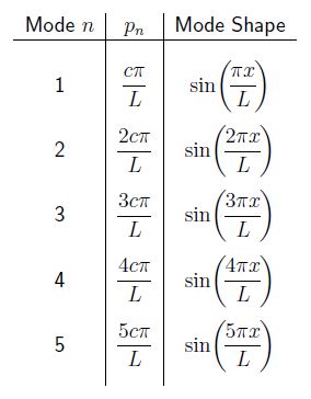
The values given by 10.11 are the natural frequencies of the system. Each natural frequency  is associated with a particular mode shape. Upon substituting the natural frequencies from 10.11 into 10.7a we obtain

or
(10.12) 
10.12 describes the  mode shape for the cable. As with discrete systems, when the cable is vibrating in one of its modes, each point on the cable undergoes simple simultaneous harmonic motion at the frequency . Each point on the cable vibrates with an amplitude proportional to the value of
  at that point. The lowest natural frequency,
  is again known as the fundamental frequency and the associated mode shape
  is known as the fundamental mode.
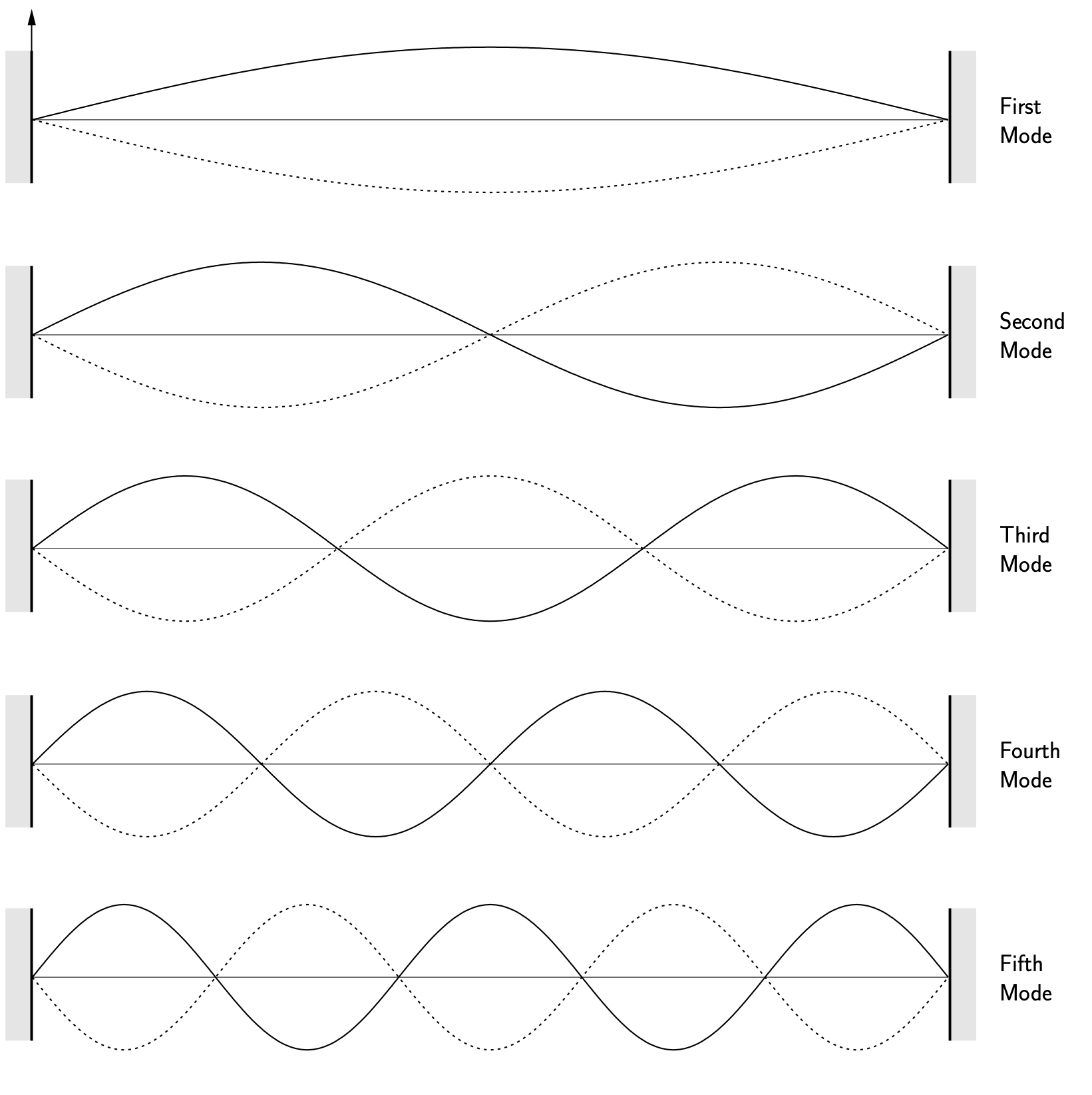
Table 10.1 lists the first five natural frequencies and mode shapes for the cable. These mode shapes are illustrated in Figure 10.2.
Complete Response of The Cable
We have found an infinite number of solutions to the wave equation 10.2 given by equations 10.8, 10.11 and 10.12 as
(10.13) ![\begin{equation*}y_n(x,t) = \sin\biggl (\frac{n \pi x}{L}\biggr)\biggl[ \hat{C}_n \, \sin\biggl (\frac{n \ensuremath{c} \pi}{L} t\biggr) +\hat{D}_n \, \cos\biggl (\frac{n \ensuremath{c} \pi}{L} t\biggr) \biggr],\qquad n = 1,2, ... \infty\end{equation*}](https://engcourses-uofa.ca/wp-content/ql-cache/quicklatex.com-d4edd1fa8d12a717bff712322b63e60b_l3.png "Rendered by QuickLaTeX.com")
Note: We have assumed that the constant is 1 without any loss of generality.
Since the wave equation is linear, the general solution to the equation of motion 10.2 is a superposition of all of the responses in 10.13,
(10.14) ![\begin{align*}y(x,t) =& \sum_{n=1}^{\infty} y_n(x,t) \nonumber \\y(x,t) =& \sum_{n=1}^{\infty}\sin\biggl (\frac{n \pi x}{L}\biggr )\biggl[ \hat{C}_n \, \sin\biggl (\frac{n \ensuremath{c} \pi}{L} t\biggr) +\hat{D}_n \, \cos\biggl (\frac{n \ensuremath{c} \pi}{L} t\biggr)\biggr]\end{align*}](https://engcourses-uofa.ca/wp-content/ql-cache/quicklatex.com-56a51a64de046fdd215f662fc87edd74_l3.png "Rendered by QuickLaTeX.com")
The constants  and
and  can be determined from the initial conditions of the cable. Note that if was not assumed to be 1 in 10.13 then here we would instead determine the constants
  and
and  . If the initial displacement and velocity of the cable are specified by
(10.15) 
(10.16) 
then 10.14 gives

and can then be found from
(10.17) 
(10.18) 
which takes advantage of the orthogonality property of the sine function

Note that as with discrete systems, the modes which participate in the response are determined entirely by the initial conditions. If the cable is started in one of its mode shapes, it will vibrate solely in that mode at the associated natural frequency.
Alternate Solution to the Wave Equation
As we have seen, the separation of variables technique can be used to find the solution to the wave equation. There is another equivalent way of looking at the solution which is known as the traveling wave solution.
Due to the form of the wave equation in 10.2

any arbitrary functions of the form

automatically satisfy the wave equation. To see this, note that
![\[\frac{\partial y_1}{\partial x} = \frac{d y_1}{d (x-\ensuremath{c} t)}\cancelto{1}{\frac{\partial (x-\ensuremath{c} t)}{\partial x}} = y_1'\]](https://engcourses-uofa.ca/wp-content/ql-cache/quicklatex.com-1aacc66130bbe65976e8061f2d951923_l3.png "Rendered by QuickLaTeX.com")
and similarly

Also,
![\[\frac{\partial y_1}{\partial t} = \frac{d y_1}{d (x-\ensuremath{c} t)}\cancelto{-c}{\frac{\partial (x-\ensuremath{c} t)}{\partial t}} = -\ensuremath{c} \,y_1'\]](https://engcourses-uofa.ca/wp-content/ql-cache/quicklatex.com-038864d90be7a5e75d9c158eec772fcf_l3.png "Rendered by QuickLaTeX.com")
and

As a result, the wave equation can be seen to be satisfied. A similar procedure can be used to show that  also satisfies the wave equation.
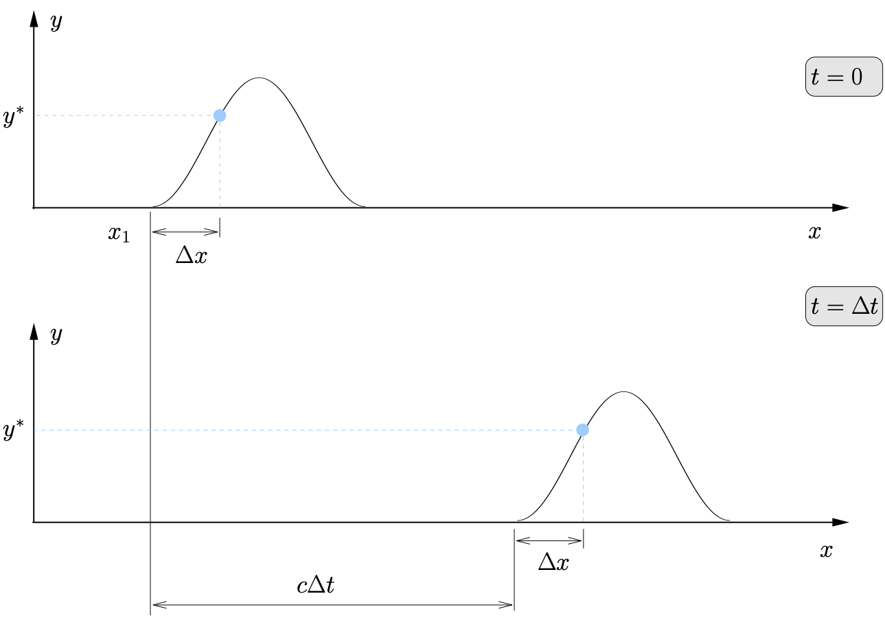
An arbitrary function  is shown in Figure 10.3, which represents a wave traveling to the right (assuming positive is to the right) at a constant speed
  with no change in the shape of the wave. If at some position and time (the top figure) the lateral deformation of the cable is
  , then at some time
  later, the cable at position
  (bottom figure) will have the same lateral deflection since

Similarly, a function of the form  represents a wave traveling to the left at a constant speed without a change in shape.
Since the wave equation is linear, the total solution will be a superposition of these two solutions

where the specific forms of and must be determined from the initial conditions of the cable. For cables of finite length, a means to account for the boundary conditions is required, which generally affect how waves “reflect” from each end. This is beyond the scope of this course.