Engineering at Alberta Courses

Transient Vibrations: Convolution

The method of convolution is based upon the response to an impulse load. We have shown previously in equation (7.4) that the response to an impulse applied at time $t=0$ is

$\begin{equation*}x(t) = \frac{F_0 \Delta t}{m p} \sin{pt}, \qquad t > 0\end{equation*}$

where $F_0 \Delta t$ is the magnitude of the impulse. To proceed, we next need to consider the response of the system due to an impulse that is applied at some other time $t'$ .

This image has an empty alt attribute; its file name is ImpulseLoadingB-300x173.jpg — Figure 7.8: Impulse applied at time $t'$

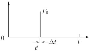
We are interested in the response of the mass at some later time $t$ , where $t>t'$ . In such a case the response of the mass at time $t$ due to an impulse applied at an earlier time $t'$ is simply

(7.9) $\begin{equation*}x(t) = \frac{F_0 \Delta t}{m p} \sin{(p(t-t'))},\qquad t>t'\end{equation*}$

where $t-t'$ is the elapsed time after the impulse was applied. Note that this assumes that the mass is at rest at time $t'$ (ie $x(t')=0$ and $\dot{x}(t')=0$ ). Equation (7.9) then gives us the position of the mass $x(t)$ at time $t$ , which is after the impulse has been applied. Note that with the assumed initial conditions, the response of the mass if the impulse were not applied would be simply $x(t) = 0$ . Therefore, what (7.9) in fact represents is the change in the response $x(t)$ , compared to what would have occurred if the impulse had not been applied.

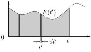
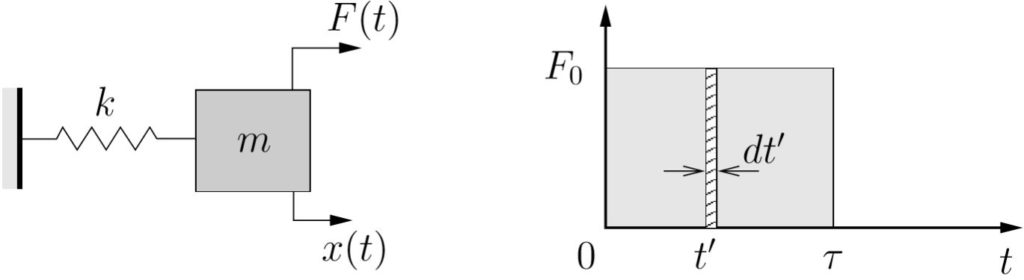
Figure 7.9: Forcing function represented as a series of impulses

Finally, consider some arbitrary forcing function $F(t)$ as shown in Figure 7.9. This function can be considered to be composed of an infinite number of infinitesimal impulsive loads, a few of which are illustrated. Again, we are interested in the response of the mass at some arbitrary time $t$ . This response will be affected by all of the impulses that have been applied up to time $t$ . Consider one such impulse at time $t'$ . The application of the impulse $F(t') dt'$ at $t'$ will have an effect on the position of the mass for all later times $t>t'$ , with the change in the position of the mass at time $t$ given by

$\begin{align*}\label{eq:ImpulseResponseTP}dx &= \frac{F(t') dt'}{m p} \sin{(p(t-t'))} \\[2mm]dx &= \frac{F(t')}{m p} \sin{(p(t-t'))} dt'\end{align*}$

exactly analogous to our previous results. As discussed previously, this actually represents the change in the response due to the application of this one impulse. To find the actual position of the mass at time $t$ , we simply add up (ie integrate) the effects of all the individual impulses up to time $t$ , which are the only ones that can affect the position at time $t$ . As a result, we get

(7.10) $\begin{equation*}\boxed{x(t) = \frac{1}{m p} \int_0^t F(t') \sin{(p(t-t'))} dt'}\end{equation*}$

(Note that $t'$ is simply a dummy variable.) Equation (7.10) is known as Duhamel’s Integral and is a special form of the convolution integral which gives the position $x(t)$ for an arbitrary load $F(t)$ . As discussed, this assumes that the initial conditions are

$\begin{equation*}x(0) = 0 \qquad\text{and}\qquad \dot{x}(0) = 0\end{equation*}$

If instead we have more general initial conditions given by

$\begin{equation*}x(0) = x_0, \qquad \dot{x}(0) = v_0\end{equation*}$

then (7.10) must be replaced by the more general form

(7.11) $\begin{equation*}\label{eq:ConvolutionIntegralGeneral}x(t) = \underbrace{\frac{v_0}{p} \sin{pt} + x_0 \cos{pt} \rule[-10mm]{0pt}{0pt}}_{\stackrel{\text{\small Response of system at time $t$}}{\text{\small if impulses were not applied}}} +\underbrace{\frac{1}{m p} \int_0^t F(t') \sin{(p(t-t'))} dt'\rule[-10mm]{0pt}{0pt}}_{\stackrel{\text{\small Change in the response due to the}}{\text{\small cumulative effect of the impulses}}}\end{equation*}$

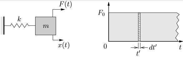
EXAMPLE

A mass, initially at rest, is subject to a step load as shown below. Determine the response of the system $x(t)$ for $t>0$ . Use the method of convolution.

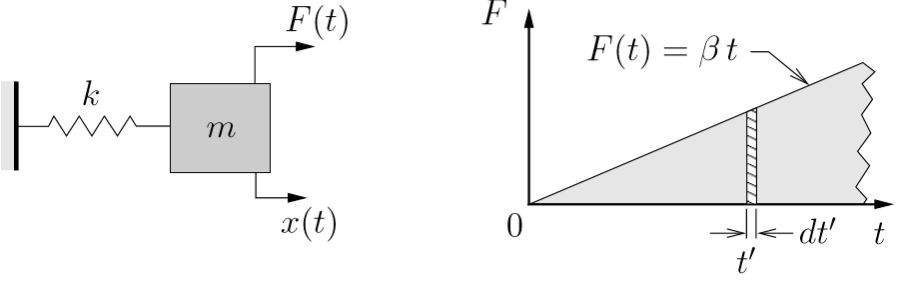
EXAMPLE

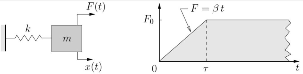
A mass, initially at rest, is subject to a ramp load as shown below. Determine the response of the system $x(t)$ for $t>0$ . Use the method of convolution.

This image has an empty alt attribute; its file name is EX2-7.jpg

EXAMPLE

A mass, initially at rest, is subject to a rectangular step load as shown below. Using the the method of convolution, determine the response of the system $x(t)$ for
a) $0 \leq t \leq \tau$
b) $t > \tau$

EXAMPLE

A mass, initially at rest, is subject to a forcing function shown below. Using the the method of convolution, determine the response of the system $x(t)$ for
a) $0 \leq t \leq \tau$
b) $t > \tau$

EXAMPLE

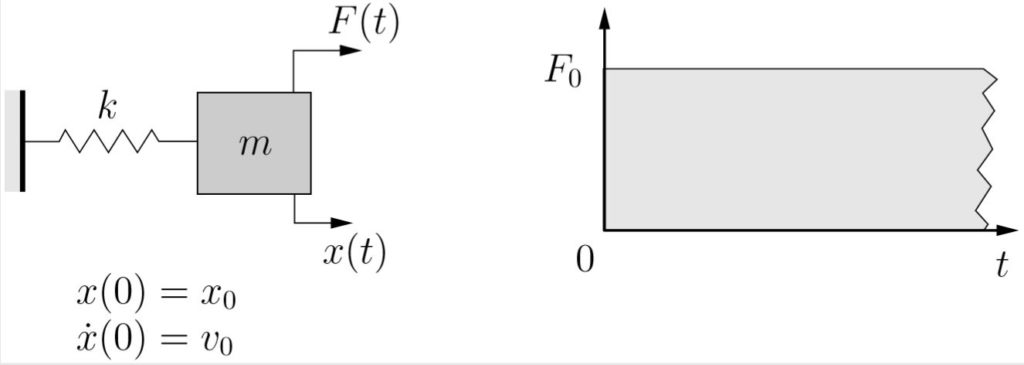
A mass is initially moving such that at some time $t=0$ the mass has position $x_0$ and velocity $v_0$ . At that instant a step load is applied to the mass as shown below.

Determine the response of the system $x(t)$ for $t>0$ using
a) Newton’s laws directly
b) The method of convolution.

Convolution with Base Excitation

In some situations we do not apply a force directly to the mass but instead the base supporting the mass is given some motion $y(t)$ . We have already seen that the equation of motion in such a case is

$\begin{equation*}m \ddot{x} + k x = k y(t)\end{equation*}$

This is identical to the equation of motion in equation (7.1) with $F(t)$ replaced by $k y(t)$ . As a result, all of our previous results can be applied. In particular, Duhamel’s Integral (equation (7.10)) becomes

$\begin{split}x(t) &= \frac{1}{m p} \int_0^t F(t') \sin{(p(t-t'))}dt' \\&= \frac{1}{m p} \int_0^t \bigl( k y(t') \bigr) \sin{(p(t-t'))}dt' \\&= \frac{k}{m p} \int_0^t y(t') \, \sin{(p(t-t'))}dt'\end{split}$

or, since $\dfrac{k}{m} = p^2$ ,

(7.12) $\begin{equation*}\boxed{x(t) = p \int_0^t y(t') \, \sin{(p(t-t'))} dt'}\end{equation*}$

Convolution with Viscous Damping

So far we have only considered undamped situations. We will now consider the response of a spring–mass system with a viscous damper subjected to an impulsive load. We will again assume the initial conditions are

$\begin{equation*}x(0) = 0, \qquad\text{and}\qquad \dot{x}(0) = 0\end{equation*}$

before any impulses are applied. Similar to the undamped case, the initial conditions just after the impulse has been applied are

$\begin{equation*}x(0) = 0, \qquad \dot{x}(0) = \frac{F_0 \Delta t}{m}\end{equation*}$

The subsequent free vibration response is given by

$\begin{equation*}x(t) = e^{-\zeta p t} \Bigl[ A \sin{\sqrt{1-\zeta^2}pt} + B \cos{\sqrt{1-\zeta^2}pt} \Bigr]\end{equation*}$

With the given initial conditions, we find that

$\begin{equation*}A = \frac{F_0 \Delta t}{m p \sqrt{1-\zeta^2}}, \qquad B = 0\end{equation*}$

so that the response becomes

$\begin{equation*}\label{eq:ImpulseResponseDamped}x(t) = \frac{F_0 \Delta t}{m p \sqrt{1-\zeta^2}} \, e^{-\zeta p t} \sin{(\sqrt{1-\zeta^2}pt)}\end{equation*}$

If the impulse were instead applied at some later time $t'$ , the response would be

$\begin{equation*}\label{eq:ImpulseResponseDamped}x(t) = \frac{F_0 \Delta t}{m p \sqrt{1-\zeta^2}} \, e^{-\zeta p \left(t-t'\right)}\sin \left(\sqrt{1-\zeta^2}p\bigl(t-t'\bigr)\right), \qquad t>t'\end{equation*}$

Now as before we consider an arbitrary forcing function to be composed of an infinite number of infinitesimal impulses. The response at time $t$ due to the impulse applied at some earlier time $t'$ is

$\begin{equation*}\label{eq:ImpulseResponseDamped}dx = \frac{F(t') d t'}{m p \sqrt{1-\zeta^2}} \, e^{-\zeta p \left(t-t'\right)}\sin \left(\sqrt{1-\zeta^2}p\bigl(t-t'\bigr)\right), \qquad t>t'\end{equation*}$

The total response at $t$ is the cumulative effect of all the impulses applied up to time $t$ , i.e.

$\begin{equation*}\boxed{x(t) = \int_0^t F(t') \, \frac{e^{-\zeta p \left(t-t'\right)}}{m p \sqrt{1-\zeta^2}} \sin \left(\sqrt{1-\zeta^2}p\bigl(t-t'\bigr)\right) \, dt'}\end{equation*}$