Engineering at Alberta Courses » Forced Vibrations of Undamped Two Degree of Freedom Systems

Multiple Degree of Freedom Systems: Forced Vibrations of Undamped Two Degree of Freedom Systems

The general form of the equations of motion for an undamped two degree of freedom system
subjected to external loading are

$\begin{bmatrix}m_{11} & m_{12} \\m_{21} & m_{22} \\\end{bmatrix}\!\!\biggl\{\!\!\!\begin{array}{c}\ddot{x}_1 \\ \ddot{x}_2 \\\end{array}\!\!\!\biggr\}+\begin{bmatrix}k_{11} & k_{12} \\k_{21} & k_{22} \\\end{bmatrix}\!\!\biggl\{\!\!\!\begin{array}{c}x_1 \\ x_2 \\\end{array}\!\!\!\biggr\}=\biggl\{\!\!\!\begin{array}{c}F_1(t) \\ F_2(t)\\\end{array}\!\!\!\biggr\}$

The solution to this general form of the equations of motion is beyond the scope of this course (but only slightly). However, we will consider a special case in which the forcing functions $F_1(t)$ and $F_2(t)$ are harmonic, at the same frequency and in-phase with each other. In such a case the equations of motion become

(8.34) $\begin{bmatrix}m_{11} & m_{12} \\m_{21} & m_{22} \\\end{bmatrix}\!\!\biggl\{\!\!\!\begin{array}{c}\ddot{x}_1 \\ \ddot{x}_2 \\\end{array}\!\!\!\biggr\}+\begin{bmatrix}k_{11} & k_{12} \\k_{21} & k_{22} \\\end{bmatrix}\!\!\biggl\{\!\!\!\begin{array}{c}x_1 \\ x_2 \\\end{array}\!\!\!\biggr\}=\biggl\{\!\!\!\begin{array}{c}F_1 \\ F_2 \\\end{array}\!\!\!\biggr\} \ensuremath{\sin\left(\omega t + \phi\right)}$

$\ensuremath{\bigl[m\bigr]}\!\ensuremath{\bigl\{\ddot{x}\bigr\}} + \ensuremath{\bigl[k\bigr]}\!\ensuremath{\bigl\{x\bigr\}} = \ensuremath{\bigl\{F\bigr\}} \ensuremath{\sin\left(\omega t + \phi\right)}$

To find the steady–state response of the system, we again look for solutions in which the masses are undergoing simple simultaneous harmonic motion at the forcing frequency

$\biggl\{\!\!\!\begin{array}{c}x_1 \\ x_2 \\\end{array}\!\!\!\biggr\}=\biggl\{\!\!\!\begin{array}{c}\mathbb{A}_1 \\ \mathbb{A}_2 \\\end{array}\!\!\!\biggr\}\sin{(\omega t + \phi)}\text{ or }\big\{x\big\} = \big\{\mathbb{A}\big\}\sin{(\omega t + \phi)}$

The equations of motion become

$-\omega^2[m]\big\{\mathbb{A}\big\}\sin{(\omega t + \phi)} +[k]\big\{\mathbb{A}\big\}\sin{(\omega t + \phi)} =\big\{F\big\}\sin{(\omega t + \phi)}$

which to be valid for all times $t$ requires

(8.35) $\Bigl[ \ensuremath{\bigl[k\bigr]} -\omega^2 \ensuremath{\bigl[m\bigr]} \Bigr] \ensuremath{\bigl\{\!\ensuremath{\mathbb{A}}\!\bigr\}} = \ensuremath{\bigl\{F\bigr\}}$

$\ensuremath{\bigl[\mathcal{Z}\bigr]}\!\!\ensuremath{\bigl\{\!\ensuremath{\mathbb{A}}\!\bigr\}} = \ensuremath{\bigl\{F\bigr\}} \nonumber$

where $\ensuremath{\bigl[\mathcal{Z}\bigr]}$ is defined as

$\ensuremath{\bigl[\mathcal{Z}\bigr]} = \ensuremath{\bigl[k\bigr]} - \omega^2 \ensuremath{\bigl[m\bigr]} =\begin{bmatrix}\mathcal{Z}_{11} & \mathcal{Z}_{12} \\\mathcal{Z}_{21} & \mathcal{Z}_{22} \\\end{bmatrix}=\begin{bmatrix}k_{11} - \omega^2 m_{11} & k_{12} - \omega^2 m_{12} \\k_{21} - \omega^2 m_{21} & k_{22} - \omega^2 m_{22} \\\end{bmatrix}$

Unlike the free vibration situation, the RHS of equation (8.35) is not zero, so that a unique solution for the amplitudes of each of the masses can be found as

(8.36) $\ensuremath{\bigl\{\!\ensuremath{\mathbb{A}}\!\bigr\}} = \ensuremath{\bigl[\mathcal{Z}\bigr]\!\!\rule[5mm]{0pt}{0pt}^{-1}}\!\!\ensuremath{\bigl\{F\bigr\}}$

which is valid provided $\det \ensuremath{\bigl[\mathcal{Z}\bigr]} \neq 0$ . Since $\ensuremath{\bigl[\mathcal{Z}\bigr]}$ is a $2\times2$ matrix, the inverse is

$\ensuremath{\bigl[\mathcal{Z}\bigr]\!\!\rule[5mm]{0pt}{0pt}^{-1}} = \frac{1}{\mathcal{Z}_{11}\mathcal{Z}_{22}-\mathcal{Z}_{12}\mathcal{Z}_{21}}\biggl[\!\!\begin{array}{rr}\mathcal{Z}_{22} & -\mathcal{Z}_{12} \\-\mathcal{Z}_{21} & \mathcal{Z}_{11} \\\end{array}\!\!\biggr]$

so we see from equation (8.36) that the steady–state amplitudes of the response a

(8.37) $\biggl\{\!\!\!\begin{array}{c}\mathbb{A}_1 \\ \mathbb{A}_2 \\\end{array}\!\!\!\biggr\}=\frac{1}{\mathcal{Z}_{11}\mathcal{Z}_{22}-\mathcal{Z}_{12}\mathcal{Z}_{21}}\biggl\{\!\!\!\begin{array}{c}\mathcal{Z}_{22}F_1 - \mathcal{Z}_{12}F_2 \\-\mathcal{Z}_{21}F_1 + \mathcal{Z}_{11}F_2\\\end{array}\!\!\!\biggr\}$

with

$\begin{align*}\mathcal{Z}_{11} &= k_{11} - m_{11}\omega^2\\\mathcal{Z}_{12} &= k_{12} - m_{12}\omega^2\\\mathcal{Z}_{21} &= k_{21} - m_{21}\omega^2\\\mathcal{Z}_{22} &= k_{22} - m_{22}\omega^2\end{align*}$

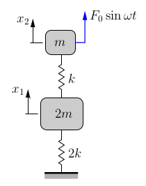
EXAMPLE

Determine the steady state response for the system shown.

Vibration Absorber

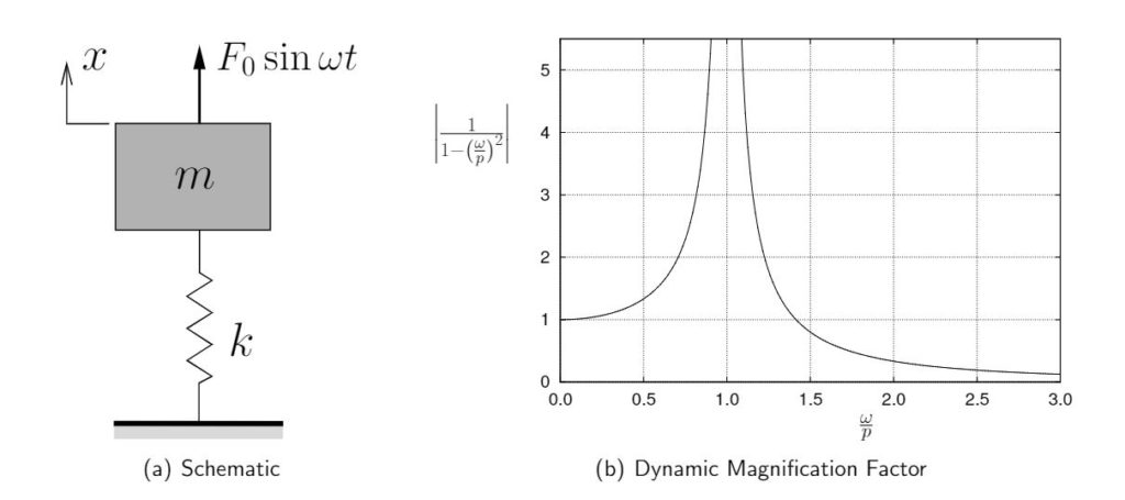
Figure 8.12: Machine undergoing excessive vibrations

As we have discussed, a machine (such as illustrated schematically in Figure 8.12(a)) may experience excessive vibrations if it is acted upon by a harmonic force at a frequency near its own natural frequency. Figure 8.12(b) shows the dynamic magnification factor for this system and illustrates the large amplitudes that can occur near resonance. To reduce these vibrations, we can try to add mass, change the spring stiffness, add damping, change the operating speed if possible, etc. Another possibility to eliminate the vibrations is to add a vibration absorber to the system as illustrated in Figure 8.13.

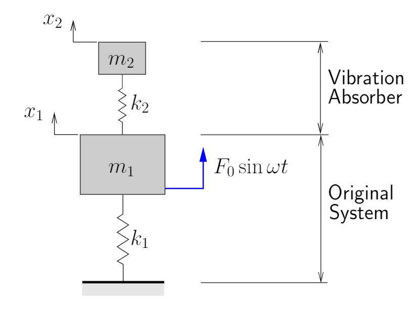
Figure 8.13: Schematic of a vibration absorber

A vibration absorber is simply an additional spring–mass system added to the original system. We would like to select the parameters for the vibration absorber ( $m_2,k_2$ ) to help minimize the vibration levels (i.e. minimize $x_1$ ) in the original system.

Figure 8.14: FBD/MAD’s for vibration absorber and original system

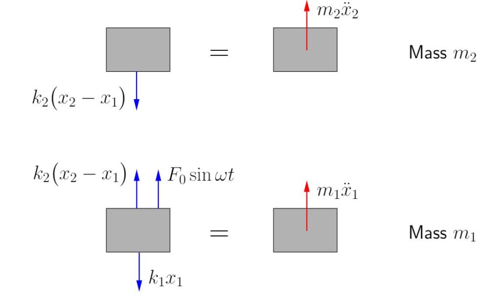
Figure 8.14 shows the FBD/MAD for the vibration absorber and the original system. The equation of motion for mass $m_1$ is

$\begin{align*}\uparrow\sum F = ma: \qquad\qquad F_0 \sin(\omega t) + k_2 ( x_2 - x_1 \bigr) - k_1 x_1 &= m_1 \ddot{x}_1, \\ m_1 \ddot{x}_1 + \bigl( k_1 + k_2 \bigr) x_1 -k_2 x_2 &= F_0 \sin(\omega t)\end{align*}$

while for the absorber we get

$\begin{align*}+\!\!\uparrow\sum F = ma: \qquad\qquad-k_2 ( x_2 - x_1 \bigr) &= m_2 \ddot{x}_2 \\m_2 \ddot{x}_2 - k_2 x_1 + k_2 x_2 &= 0\end{align*}$

In matrix form these can be written as

(8.38) $\begin{equation*}\begin{bmatrix} m_1 & 0 \\ 0 & m_2 \\ \end{bmatrix}\!\! \biggl\{\!\!\! \begin{array}{c} \ddot{x}_1 \\ \ddot{x}_2 \\ \end{array} \!\!\!\biggr\} + \begin{bmatrix} k_1+k_2 & -k_2 \\ -k_2 & \phantom{-}k_2 \\ \end{bmatrix}\!\! \biggl\{\!\!\! \begin{array}{c} x_1 \\ x_2 \\ \end{array} \!\!\!\biggr\} = \biggl\{\!\!\! \begin{array}{c} F_0 \\ 0 \\ \end{array} \!\!\!\biggr\} \sin(\omega t)}\end{equation*}$

(Note that this is a special case of (8.34) with $F_2= 0$ .)

We look for solutions of the form

$\begin{equation*}\biggl\{\!\!\! \begin{array}{c} x_1 \\ x_2 \\ \end{array} \!\!\!\biggr\} = \biggl\{\!\!\! \begin{array}{c} \mathbb{X}_1 \\ \mathbb{X}_2 \\ \end{array} \!\!\!\biggr\} \, \sin(\omega t)\end{equation*}$

With this, the equations of motion become

$\begin{equation*}-\omega^2 \begin{bmatrix} m_1 & 0 \\ 0 & m_2 \\ \end{bmatrix}\!\! \biggl\{\!\!\! \begin{array}{c} \mathbb{X}_1 \\ \mathbb{X}_2 \\ \end{array} \!\!\!\biggr\} \cancel{\sin(\omega t)} + \biggl[\!\! \begin{array}{cc} k_1+k_2 & -k_2 \\ -k_2 & \phantom{-}k_2 \\ \end{array} \!\!\biggr]\!\! \biggl\{\!\!\! \begin{array}{c} \AMP_1 \\ \AMP_2 \\ \end{array} \!\!\!\biggr\} \cancel{\sin(\omega t)} = \biggl\{\!\!\! \begin{array}{c} F_0 \\ 0 \\ \end{array} \!\!\!\biggr\} \cancel{\sin(\omega t)}\end{equation*}$

which to be valid for all times $t$ requires

$\begin{equation*}-\omega^2 \begin{bmatrix} m_1 & 0 \\ 0 & m_2 \\ \end{bmatrix}\!\! \biggl\{\!\!\! \begin{array}{c} \mathbb{X}_1 \\ \mathbb{X}_2 \\ \end{array} \!\!\!\biggr\} + \biggl[\!\! \begin{array}{cc} k_1+k_2 & -k_2 \\ -k_2 & \phantom{-}k_2 \\ \end{array} \!\!\biggr]\!\! \biggl\{\!\!\! \begin{array}{c} \mathbb{X}_1 \\ \mathbb{X}_2 \\ \end{array} \!\!\!\biggr\} = \biggl\{\!\!\! \begin{array}{c} F_0 \\ 0 \\ \end{array} \!\!\!\biggr\}\end{equation*}$

(8.39) $\begin{equation*}\begin{bmatrix} k_1+k_2 -m_1 \omega^2 & -k_2 \\ -k_2 & k_2 -m_2 \omega^2 \\ \end{bmatrix}\!\! \biggl\{\!\!\! \begin{array}{c} \mathbb{X}_1 \\ \mathbb{X}_2 \\ \end{array} \!\!\!\biggr\} = \biggl\{\!\!\! \begin{array}{c} F_0 \\ 0 \\ \end{array} \!\!\!\biggr\}\end{equation*}$

To solve for the steady–state vibration amplitudes, we can see from the second equation that

$\begin{equation*} -k_2 \mathbb{X}_1 + (k_2 - m_2 \omega^2) \mathbb{X}_2 = 0\end{equation*}$

(*) $\begin{equation*} \mathbb{X}_2 = \frac{k_2}{k_2-m_2 \omega^2} \mathbb{X}_1\end{equation*}$

With this result the first equation becomes

$\begin{equation*} \bigl( k_1+k_2 -m_1 \omega^2 \bigr) \mathbb{X}_1 -k_2 \biggl[ \frac{k_2}{k_2-m_2 \omega^2} \mathbb{X}_1 \biggr] = F_0\end{equation*}$

which can be solved for $\mathbb{X}_1$

(8.40) $\begin{equation*} \mathbb{X}_1 = \frac{F_0 \bigl(k_2-m_2 \omega^2 \bigr)}{\bigl( k_1+k_2 - m_1 \omega^2 \bigr)\bigl(k_2 - m_2 \omega^2 \bigr) - k_2^2}\end{equation*}$

and upon substitution of this result into (*) we also find

(8.41) $\begin{equation*} \mathbb{X}_2 = \frac{F_0 k_2}{\bigl( k_1+k_2 - m_1 \omega^2 \bigr)\bigl(k_2 - m_2 \omega^2 \bigr) - k_2^2}\end{equation*}$

Note that these are the same results we would have obtained had we applied (8.36) directly.

To help non–dimensionalize these results, we divide the top and bottom of equation (8.40) and (8.41) by $k_1k_2$

$\begin{align*} \mathbb{X}_1 &= \dfrac{\dfrac{F_0}{k_1} \left(1-\frac{m_2}{k_2} \omega^2 \right)}{\left( 1+ \dfrac{k_2}{k_1} - \dfrac{m_1}{k_1} \omega^2 \right)\left(1 - \dfrac{m_2}{k_2} \omega^2 \right) - \dfrac{k_2}{k_1}} \\ \mathbb{X}_2 &= \dfrac{\dfrac{F_0}{k_1}}{\left( 1+ \dfrac{k_2}{k_1} - \dfrac{m_1}{k_1} \omega^2 \right)\left(1 - \dfrac{m_2}{k_2} \omega^2 \right) - \dfrac{k_2}{k_1}}\end{align*}$

Defining

$\begin{align*}\delta_{ST} &= \frac{F_0}{k_1} \quad - \quad \text{Static deflection of original system}\\p^2_{11} &= \frac{k_1}{m_1} \quad - \quad \text{Natural frequency of the original system}\\p^2_{22} &= \frac{k_2}{m_2} \quad - \quad \text{Natural frequency of vibration absorber in isolation}\\\mu &= \frac{m_2}{m_1} \quad - \quad \text{Mass ratio}\end{align*}$

these can be written

(8.42a) $\begin{equation*}\dfrac{\mathbb{X}_1}{\delta_{ST}} &= \dfrac{1-\left(\frac{\omega}{p_{22}}\right)^2} {\biggl[ 1 + \mu (\frac{p_{22}}{p_{11}})^2 - (\frac{\omega}{p_{11}})^2 \biggr]\biggl[1 - (\frac{\omega}{p_{22}})^2\biggr]-\mu(\frac{p_{22}}{p_{11}})^2}\end{equation*}$

(8.42b) $\begin{equation*}\dfrac{\mathbb{X}_2}{\delta_{ST}} &= \dfrac{1} {\biggl[ 1 + \mu (\frac{p_{22}}{p_{11}})^2 - (\frac{\omega}{p_{11}})^2 \biggr]\biggl[1 - (\frac{\omega}{p_{22}})^2\biggr]-\mu(\frac{p_{22}}{p_{11}})^2}\end{equation*}$

where we have used the fact that

$\begin{equation*} \frac{k_2}{k_1} = \frac{p_{22}^2 m_2}{p_{11}^2 m_1} = \mu \left(\frac{p_{22}}{p_{11}}\right)^2\end{equation*}$

Note that $p_{11}$ and $p_{22}$ are the natural frequencies of the original system and the vibration absorber each in isolation. These are not the two natural frequencies of the combined system. Those will be discussed shortly.

From equation (8.42a) we can see that the amplitude of vibration of the original mass will be zero if we select the natural frequency of the vibration absorber to be equal to the forcing frequency ( $p_{22}=\omega$ ). This is the ultimate goal of the vibration absorber. Note that in doing so, the amplitude of the motion of the vibration absorber itself is not zero but from equation (8.42b) is

$\begin{equation*} \mathbb{X}_2 = \dfrac{\delta_{ST}} {\biggl[ 1 + \mu \left(\frac{p_{22}}{p_{11}}\right)^2 - \left(\frac{\omega}{p_{11}}\right)^2 \biggr]\biggl[1 - \left(\frac{\omega}{p_{11}}\right)^2\biggr]-\mu\left(\frac{p_{22}}{p_{11}}\right)^2}\end{equation*}$

so that

$\begin{equation*} \mathbb{X}_2 = \dfrac{\delta_{ST}}{-\mu \left(\frac{p_{22}}{p_{11}}\right)^2} = \dfrac{\dfrac{F_0}{\cancel{k_1}}}{-\dfrac{k_2}{\cancel{k_1}}}\end{equation*}$

(8.43) $\begin{equation*} \boxed{\mathbb{X}_2 = -\frac{F_0}{k_2}}\end{equation*}$

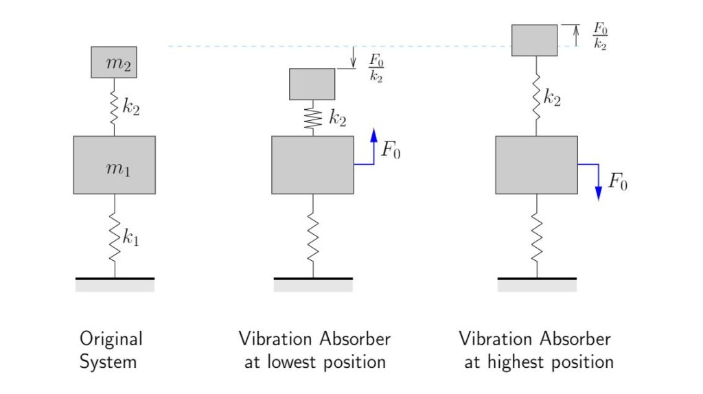
The amplitude of the motion of the vibration absorber is simply the static deflection that would result if the disturbing force were applied statically to the vibration absorber itself in isolation. The negative sign in (8.43) indicates that the absorber mass moves out of phase with the forcing function. This is illustrated in Figure 8.15. Note that the net force acting on the original mass is always in balance, resulting in no motion for the original system

Figure 8.15: Vibration absorber mass moves out of phase with the applied force (original mass is always in equilibrium and does not move)

In practice, since $\omega = p_{22} = \sqrt{\frac{k_2}{m_2}}$ , to obtain the appropriate $p_{22}$ we require
(i) a large spring constant $k_2$ and a large mass $m_2$ , or
(ii) a small spring constant $k_2$ and a small mass $m_2$ .

In the first case, a large vibration absorber mass must be used, which may be a problem. In the second case, a small mass may be used along with a light spring, but since $\mathbb{X}_2=-\frac{−F_0}{k_2}$ from (8.43), this means that the vibration absorber will undergo large motions which is also usually a problem. The choice of appropriate values for $k_2$ and $m_2$ is usually a tradeoff between these two considerations. We must also consider the effect of the vibration absorber on the natural frequencies of the combined system which we will discuss next.

Natural Frequencies of Combined System

The addition of a vibration absorber will result in no motion of the original system when $p_{22}$ is selected to be equal to the forcing frequency $\omega$ . $\omega$ (and therefore $p_{22}$ ) is not a natural frequency of the combined system, since when the combined system is excited at one of its natural frequencies, we expect the amplitude of the resulting vibrations to grow very large

In that sense, the natural frequencies of the combined system can be found easily by setting the denominator in equations (8.42a) and (8.42b) to zero

(8.44) $\begin{equation*} \biggl[ 1 + \mu \left(\frac{p_{22}}{p_{11}}\right)^2 - \left(\frac{\omega}{p_{11}}\right)^2 \biggr]\biggl[1 - \left(\frac{\omega}{p_{22}}\right)^2\biggr]-\mu\left(\frac{p_{22}}{p_{11}}\right)^2 = 0\end{equation*}$

since this implies that the amplitudes of the response grow towards infinity. The values of $\omega$ which satisfy (8.44) will therefore correspond to the natural frequencies of the combined system. (Note that we could also find the natural frequencies by considering the free vibration problem for the two degree of freedom system and using the techniques we have already discussed. This procedure will lead to exactly the same values for the natural frequencies.)

To find these natural frequencies we can expand (8.44) and substitute $p=\omega$ to find

$\begin{equation*} 1 -\left(\frac{p}{p_{22}}\right)^2 + \cancel{\mu\left(\frac{p_{22}}{p_{11}}\right)^2} -\mu\left(\frac{p_{22}}{p_{11}}\right)^2\left(\frac{p}{p_{22}}\right)^2 -\left(\frac{p}{p_{11}}\right)^2 + \left(\frac{p}{p_{11}}\right)^2\left(\frac{p}{p_{22}}\right)^2 -\cancel{\mu\left(\frac{p_{22}}{p_{11}}\right)^2} = 0\end{equation*}$

(8.45) $\begin{equation*} \left(\frac{p_{22}}{p_{11}}\right)^2\left(\frac{p}{p_{22}}\right)^4 - \biggl[ 1 + \bigl(1 + \mu \bigr)\left(\frac{p_{22}}{p_{11}}\right)^2 \biggr]\left(\frac{p}{p_{22}}\right)^2 + 1 = 0\end{equation*}$

Equation (8.45) is a quadratic equation for $(\frac{p}{p_{22}})^2$ which can be seen to depend on the quantities $p_{11}, p_{22}$ and $\mu$ . $p_{11}$ is the natural frequency of the original system and is not adjusted in selecting the vibration absorber. $p_{22}$ is the natural frequency of the vibration absorber and is usually selected to be equal to the forcing frequency $\omega$ to eliminate the vibrations of the original system. The quantity $\mu$ , however, is a parameter that can be adjusted when selecting a vibration absorber.

To illustrate the effect that $\mu$ has on the natural frequencies of the combined system, consider the case in which a vibration absorber is to be added to a system originally operating at resonance (i.e. $\omega=p_{11}$ ). Since $p_{22}$ is chosen to be $\omega$ , we also have $p_{22}=p_{11}$ . In such a case, equation (8.45) simplifies to

$\begin{equation*} \left(\frac{p}{p_{22}}\right)^4 - \biggl[ 2 + \mu \biggr] \left(\frac{p}{p_{22}}\right)^2 + 1 = 0\end{equation*}$

Figure 8.16 illustrates the effect of the parameterμon the natural frequencies of the combined system. The natural frequencies are those at which the amplitudes of the response grow towards infinity. For small values of $\mu$ ( $\mu= 0.05$ ), the two natural frequencies of the combined system remain close to the natural frequency of the original system. Therefore, although the vibration absorber should prevent the vibrations of the original system at a forcing frequency $\omega$ , if the forcing frequency is slightly different (for whatever reason) the combined system could once again be in a resonance situation. The presence of the vibration absorber in such situations could potentially make things worse compared to the original system.

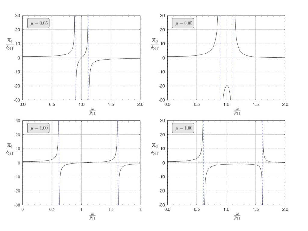
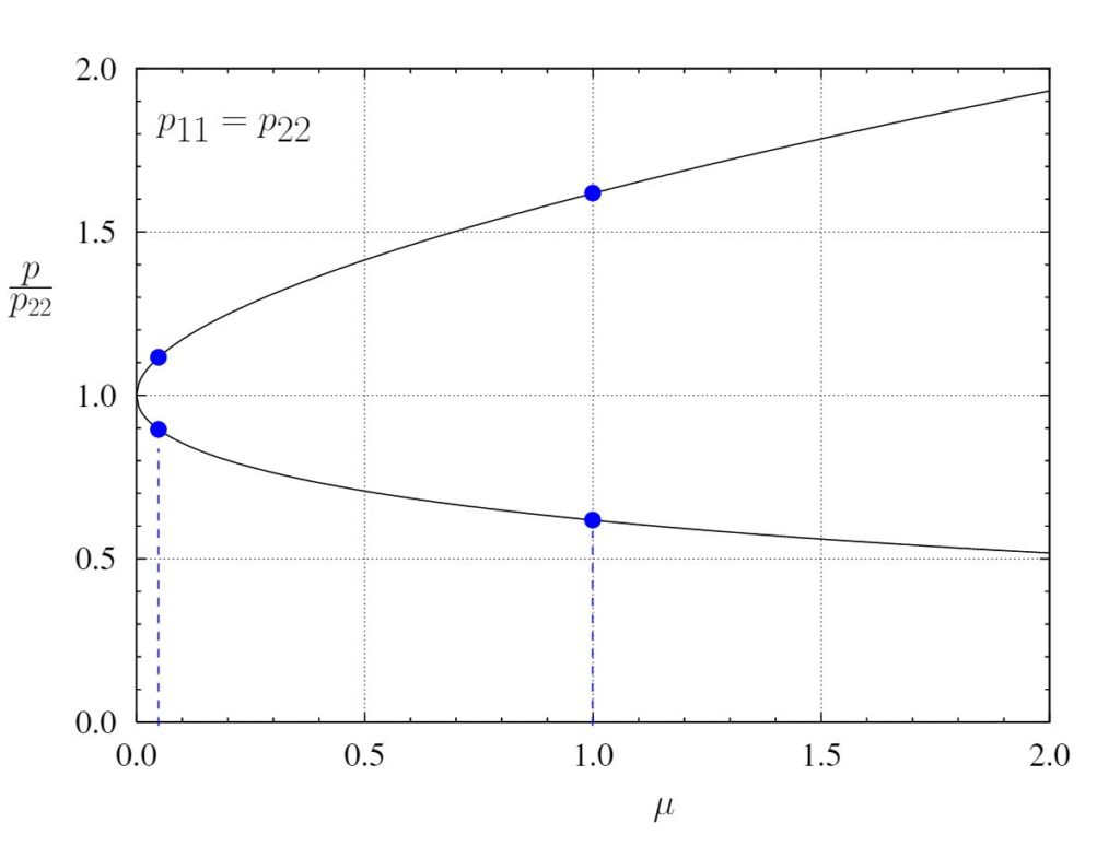
Figure 8.16: Amplitude of the response for a vibration absorber

Figure 8.17: Natural frequencies of combined system

As $\mu$ becomes larger, the natural frequencies move further away from the original natural frequency. This is also shown in Figure 8.17 which illustrates the two natural frequencies as a function of $\mu$ in this situation. As can be seen, as the mass ratio $\mu$ gets larger, the two natural frequencies of the combined system move farther apart, away from the natural frequency of the original system $p_{11}$ .

Note that the results shown are for the specific situation in which the original system is operating at resonance (so that $p_{11} = p_{22} = \omega$ ). In other situations the results will be different, but the same principles apply. Equation (8.45) can be used to find the resulting natural frequencies.

EXAMPLE

An industrial installation of process shakers shows a violent resonance when operated at 456 cycles/min. As a trial remedy, two 5 kg vibration absorbers are attached. The resulting system shows two natural frequencies occurring at 404 and 515 cycles/min.

Determine the number of vibration absorbers required to ensure that no resonance occurs between 350 and 600 cycles/min.

EXAMPLE

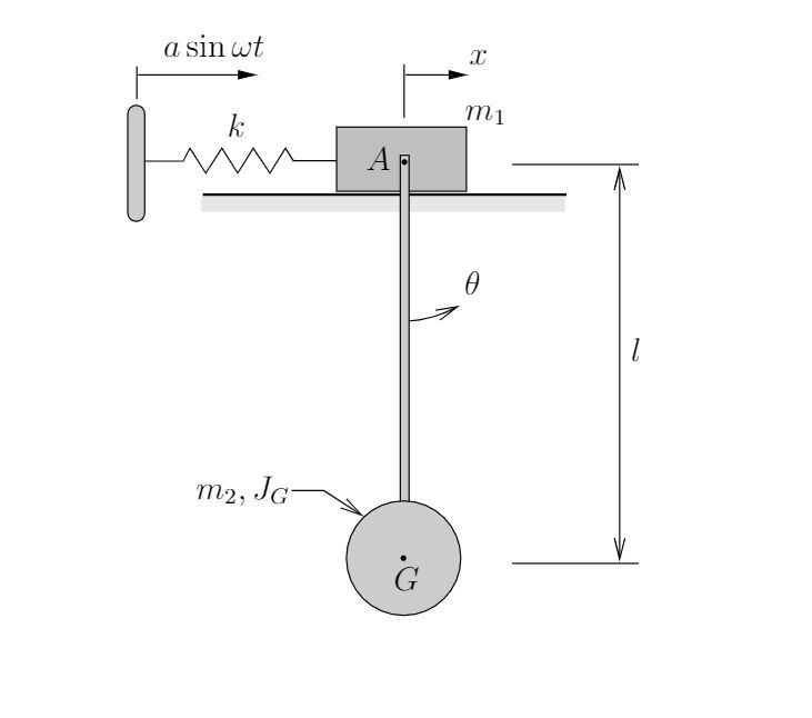
Determine the steady state response of the system shown below. Mass $m_1$ moves on a smooth horizontal surface. and is connected to a moving surface through a spring with stiffness $k$ . A pendulum of length $l$ is attached to mass $m_1$ at $A$ which is a frictionless pin.