
Approximate Methods for Multiple Degree of Freedom Systems: Rayleigh’s Quotient
For a conservative MDOF system, the total mechanical energy  is a constant so that

or using the representations in (9.1) and (9.2)
(9.3) ![\begin{equation*} \frac{1}{2} \bigl\{\!\dot{q}\!\bigr\}^{T} \!\!\bigl[m\bigr]\! \bigl\{\!\dot{q}\!\bigr\} +\frac{1}{2} \bigl\{\!q\!\bigr\}\!\rule[4mm]{0pt}{0pt}^{T} \!\!\bigl[k\bigr]\! \bigl\{\!q\!\bigr\} = E\end{equation*}](https://engcourses-uofa.ca/wp-content/ql-cache/quicklatex.com-9f5036bc1314bdc3a2428d19fe53ae82_l3.png "Rendered by QuickLaTeX.com")
Now consider the system vibrating in one of its normal modes at a natural frequency  . The amplitudes of the coordinates are given by
![\begin{equation*}\bigl\{\!q\!\bigr\}= A \bigl\{\!\Phi\!\bigr\}\!\!\rule[5mm]{5pt}{0pt} \sin\left(p t + \phi\right)\end{equation*}](https://engcourses-uofa.ca/wp-content/ql-cache/quicklatex.com-58d296ed00aa67c919e8b31935671f5e_l3.png "Rendered by QuickLaTeX.com")
where ![\bigl\{\!\Phi\!\bigr\}\!\!\rule[3mm]{0pt}{0pt}](https://engcourses-uofa.ca/wp-content/ql-cache/quicklatex.com-b1cd77a0aca1187618aa2df014cecaf6_l3.png "Rendered by QuickLaTeX.com") is the corresponding mode shape and
is the corresponding mode shape and  is a constant. The derivatives of the coordinates will therefore be
![\begin{equation*}\bigl\{\!\dot{q}\!\bigr\} = A \bigl\{\!\Phi\!\bigr\}\!\!\rule[5mm]{3pt}{0pt} \ensuremath{p} \cos\left(p t + \phi\right)\end{equation*}](https://engcourses-uofa.ca/wp-content/ql-cache/quicklatex.com-debeef6c119cedbb3abd623150241f40_l3.png "Rendered by QuickLaTeX.com")
The coordinates will have maximum values given by
(9.4) 
which all occur simultaneously (when  ). At the same instant,
  so the derivatives of the coordinates will all be zero (
 ).
).
Similarly the coordinate derivatives will have maximum values given by
(9.5) 
when  . At this instant,
  so the coordinates themselves are all zero (i.e. the system is passing through its equilibrium configuration).
In summary

Now, consider equation (9.3) at the instant when . We see that
![\begin{align*}\frac{1}{2} \bigl\{\!\dot{q}\!\bigr\}\!\rule[4mm]{0pt}{0pt}^{T} \!\!\bigl[m\bigr] \! \bigl\{\!\dot{q}\!\bigr\} +\frac{1}{2} \bigl\{\!q\!\bigr\}\!\rule[4mm]{0pt}{0pt}^{T} \!\!_{\text{MAX}}\!\bigl[k\bigr] \! \bigl\{\!q\!\bigr\}_{\text{MAX}} &= E \nonumber \\\frac{1}{2} \Bigl(A \!\bigl\{\!\Phi\!\bigr\}\!\rule[4mm]{0pt}{0pt}^{T} \!\Bigr) \!\!\bigl[k\bigr] \! \Bigl(\! A \bigl\{\!\Phi\!\bigr\} \!\Bigr) &= E\end{align*}](https://engcourses-uofa.ca/wp-content/ql-cache/quicklatex.com-0c1883c57e414c3b78d588ca92b1e5b1_l3.png "Rendered by QuickLaTeX.com")
or
(9.6) ![\begin{equation*} \frac{1}{2} A^2 \bigl\{\!\Phi\!\bigr\}\!\rule[4mm]{0pt}{0pt}^{T} \!\!\bigl[k\bigr] \! \bigl\{\!\Phi\!\bigr\} &= E.\end{equation*}](https://engcourses-uofa.ca/wp-content/ql-cache/quicklatex.com-552e723ce4aab8164a8329ea343693ee_l3.png "Rendered by QuickLaTeX.com")
Similarly, when we find
![\begin{align*}\frac{1}{2} \bigl\{\!\dot{q}\!\bigr\}_{\text{MAX}}\!\bigl[m\bigr]\! \bigl\{\!\dot{q}\!\bigr\}_{\text{MAX}} +\frac{1}{2} \bigl\{\!q\!\bigr\}\!\rule[4mm]{0pt}{0pt}^{T} \!\!\bigl[k\bigr] \! \bigl\{\!q\!\bigr\} &= E \\\frac{1}{2} \Bigl( \! A p \bigl\{\!\Phi\!\bigr\}\!\rule[4mm]{0pt}{0pt}^{T} \!\Bigr) \!\!\bigl[m\bigr] \! \Bigl(\! A p \bigl\{\!\Phi\!\bigr\} \!\Bigr) &= E\end{align*}](https://engcourses-uofa.ca/wp-content/ql-cache/quicklatex.com-00730dcc6e2ea07779a42f7e696b4044_l3.png "Rendered by QuickLaTeX.com")
or
(9.7) ![\begin{equation*} \frac{1}{2} A^2 p^2 \bigl\{\!\Phi\!\bigr\}\!\rule[4mm]{0pt}{0pt}^{T} \!\!\bigl[m\bigr] \! \bigl\{\!\Phi\!\bigr\} &= E\end{equation*}](https://engcourses-uofa.ca/wp-content/ql-cache/quicklatex.com-f0bb6d3292edbe5e34b7c947ce49bbcb_l3.png "Rendered by QuickLaTeX.com")
Since the total energy is a constant for this conservative system, comparing equations (9.6) and (9.7 ) leads to the conclusion that
![\[\cancel{\frac{1}{2}A^2}\{\Phi\}^T[k]\{\Phi\} = \cancel{\frac{1}{2}A^2}p^2\{\Phi\}^T[m]\{\Phi\}\]](https://engcourses-uofa.ca/wp-content/ql-cache/quicklatex.com-0d871a44a5e9a5ab563791c86684f1bf_l3.png "Rendered by QuickLaTeX.com")
or
(9.8) ![\begin{equation*} \boxed{p^2 = \frac{\hspace{-1cm}\bigl\{\!\Phi\!\bigr\}\!\rule[4mm]{0pt}{0pt}^{T} \!\!\bigl[k\bigr] \! \bigl\{\!\Phi\!\bigr\} \rule{-3mm}{0pt}}{\bigl\{\!\Phi\!\bigr\}\!\rule[4mm]{0pt}{0pt}^{T} \!\!\bigl[m\bigr] \! \bigl\{\!\Phi\!\bigr\} \rule{5mm}{0pt}}}\end{equation*}](https://engcourses-uofa.ca/wp-content/ql-cache/quicklatex.com-bc5d3fda54d04bb096f88151aca21024_l3.png "Rendered by QuickLaTeX.com")
Equation (9.8) is known as Rayleigh’s Quotient. This result tells us that if a mode shape corresponding to a particular natural frequency is used in the ratio in (9.8), then the result will be the associated natural frequency squared.
By itself this is not a particularly useful result since typically, knowing ![\bigl[k\bigr]](https://engcourses-uofa.ca/wp-content/ql-cache/quicklatex.com-2aab9db82919d8134feae5242052b74d_l3.png "Rendered by QuickLaTeX.com") and
and ![\bigl[m\bigr]](https://engcourses-uofa.ca/wp-content/ql-cache/quicklatex.com-733313d5e0f56bcd4cc88051f9f20e88_l3.png "Rendered by QuickLaTeX.com") for a particular system, we must find as part of the process of determining the mode shapes in the first place. However, equation (9.8) can be useful for obtaining approximate natural frequencies for MDOF systems. In essence, what we do is estimate a mode shape
for a particular system, we must find as part of the process of determining the mode shapes in the first place. However, equation (9.8) can be useful for obtaining approximate natural frequencies for MDOF systems. In essence, what we do is estimate a mode shape ![\bigl\{\!\Phi\!\bigr\}\!\!\rule[5mm]{0pt}{0pt}](https://engcourses-uofa.ca/wp-content/ql-cache/quicklatex.com-00a279fae18371111a929bdc0e89796e_l3.png "Rendered by QuickLaTeX.com") for the system and Rayleigh’s Quotient returns an associated estimate of the natural frequency. Obviously, the choice of
for the system and Rayleigh’s Quotient returns an associated estimate of the natural frequency. Obviously, the choice of ![\bigl\{\!\Phi\!\bigr\}\!\!\rule[5mm]{0pt}{0pt}{1}](https://engcourses-uofa.ca/wp-content/ql-cache/quicklatex.com-1ee1ef136a94d951f603de03e5400364_l3.png "Rendered by QuickLaTeX.com") will influence the value of the returned natural frequency, however it can be shown that if
will influence the value of the returned natural frequency, however it can be shown that if  are the
  natural frequencies on an degree of freedom system, then for any assumed mode shape the frequency returned by Rayleigh’s Quotient satisfies

i.e. the frequency returned by Rayleigh’s Quotient will always be higher than the lowest natural frequency and lower than the highest natural frequency in the system. Typically we are more concerned with the lowest (fundamental) frequency in a system, for which Rayleigh’s Quotient establishes an upper bound. (This frequency also provides a lower bound on the highest natural frequency of a system but this is usually of less interest.)
Remarkably good estimates of the fundamental natural frequency can be obtained even if the assumed mode shape (also called a trial vector) is not equal to the actual first mode shape.
EXAMPLE
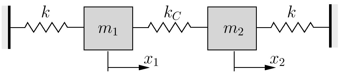
(a) For the system shown above, estimate the fundamental natural frequency using Rayleigh’s Quotient. Assume  and use trial vectors of

and comment on the results. It was previously determined that
![\[\bigl[ k \bigr] =\biggl[\! \begin{array}{cc}k+k_C & -k_C \\-k_C & k+k_C \\\end{array} \!\biggr] , \qquad\bigl[ m \bigr] =\begin{bmatrix}m & 0 \\0 & m \\\end{bmatrix}\]](https://engcourses-uofa.ca/wp-content/ql-cache/quicklatex.com-10d6e3a3a6ba95e27fd74fefa6e575d4_l3.png "Rendered by QuickLaTeX.com")
![\[p_1^2 = \frac{k}{m}, \qquad\bigl\{\!\Phi\!\bigr\}^{(1)} =\biggl\{\!\begin{array}{r}1 \\ 1 \\\end{array}\!\biggr\}, \qquad p_2^2 = \frac{k+2k_C}{m}, \qquad\bigl\{\!\Phi\!\bigr\}^{(2)} =\biggl\{\!\begin{array}{r}1 \\ -1 \\\end{array}\!\biggr\}\]](https://engcourses-uofa.ca/wp-content/ql-cache/quicklatex.com-52389163ce6a5e34f2929d10ee8b1416_l3.png "Rendered by QuickLaTeX.com")
(b) Repeat the calculations in part (a) assuming  ,
,  , and
, and  .
.
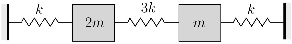
Note that the exact solution in this case is
![\[p_1 \approx 0.809 \sqrt{\frac{k}{m}}, \qquad\bigl\{\Phi\bigr\}^{\textcircled{{\footnotesize{1}}}} \approx\biggl\{ \!\begin{array}{c}1.115 \\ 1 \\\end{array}\!\biggr\} \qquad \\\]](https://engcourses-uofa.ca/wp-content/ql-cache/quicklatex.com-5506de8b1a7216d0992c42699df17a43_l3.png "Rendered by QuickLaTeX.com")
![\[p_2 \approx 2.312 \sqrt{\frac{k}{m}}, \qquad\bigl\{\!\Phi\!\bigr\}^{\textcircled{{\footnotesize{2}}}} \approx\biggl\{\!\begin{array}{c}-0.448 \\ 1 \\\end{array}\!\biggr\}\]](https://engcourses-uofa.ca/wp-content/ql-cache/quicklatex.com-6ca12d2ea14a2959ab8ebfd9858da2f6_l3.png "Rendered by QuickLaTeX.com")
EXAMPLE
Use Rayleigh’s method to estimate the fundamental natural frequency for a light simply supported beam supporting three equally spaced identical masses.
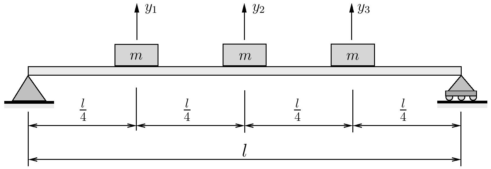
Assume trial vectors of

Note that for this problem
![\begin{align*}\bigl[ k \bigr] &=\frac{192 EI}{7 l^3}\Biggl[\begin{array}{rrr}23 & -22 & 9\\-22 & 32 & -22\\9 & -22 & 23\\\end{array}\vspace{4mm}\Biggr] \\\bigl[ m \bigr] &=m\Biggl[\begin{array}{ccc}1 & 0 & 0\\0 & 1 & 0\\0 & 0 & 1\\\end{array}\Biggr] \\\end{align*}](https://engcourses-uofa.ca/wp-content/ql-cache/quicklatex.com-e0b3cf362fb65699d432aedc2502b00d_l3.png "Rendered by QuickLaTeX.com")
Thank you. I am 82. At seven years of age I was labeled a total retard, unteachable and unlearnable by the Catholic Church. A nun, Sister Angela Cool did an experiment and I was allowed into regular class. Throughout life I have been denounced as an idiot savant. So what? We learn differently; with the main obstacle being being libeled as above; then removed from any and all stimuli including social interaction. Leave us alone. Let us learn. And we can really contribute to society and government in our own ways. That includes keeping the self-righteous, self-promoting, shady law enforcement and other such secretive organizations off our backs. My life was destroyed by two such FBI creatures, snake-headed skunks, that claimed I did not have the imagination to develop weapons and other things for the Navy. They robbed me of credit, merit, monetary awards, and my life to make themselves safe careers. Please see that it does not happen to other people like me. So I have a hobby of learniong through self research. And my country is robbed of the benefits.