
Sound and Acoustics: Fluctuating Noise Levels
In most situations, noise levels are not constant but vary continuously. The type of noise being measured, as well as the reason for taking the measurement, will influence how these fluctuating noise levels are dealt with.
Short Term Measurements
For short term measurements, to measure how loud a sound is now, most sound level meters have several basic modes they can use.
- Fast and Slow Modes
In these modes the meter determines a running time average of the square of the pressure signal (remember that the energy content in an acoustic wave is proportional to its pressure squared). The fast and slow modes correspond to the period used to determine the average. The fast mode typically corresponds to a period of 100–125 ms while the slow mode is usually between 500–1000 ms. As the names imply, the fast mode is better able to track rapidly changing noise levels while the the slow response is less sensitive to the rapid changes and produces a more stable reading. - Peak Measurement.
The peak measurement mode indicates the highest instantaneous sound pressure level experienced during a measurement. This is different from the maximum values determined using either the fast or slow modes which are averaged over some period of time. Peak values can be as much as 20 dB higher than the averaged ones.
In some cases, we are more interested in the longer term variations in the sound pressure levels, although we do not want to describe the entire sound level history as shown in Figure 12.12. There are several methods that are used to accomplish this.
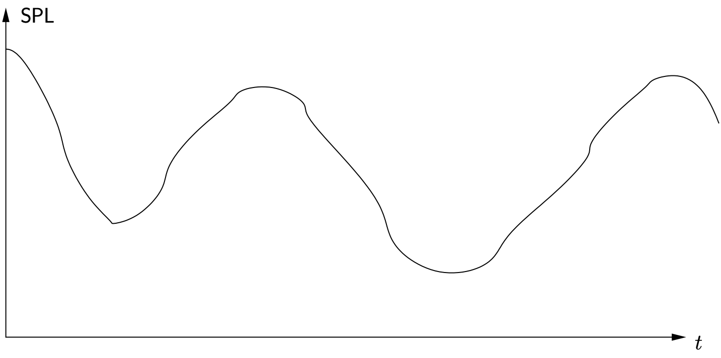
Figure 12.12: Sample long term variation in sound pressure levels
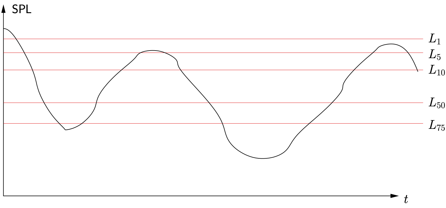
Figure 12.13: L Levels
 Levels
An level is simply the sound pressure level (typically A–weighted) that is exceeded  percent of the time, as shown in Figure 12.13. These are generally defined for periods of 15 min, 1 hour or 24 hours.
Equivalent Sound Levels (LEQ)
The equivalent sound level ( ) is defined as the constant sound level whose acoustic energy is equivalent to the acoustic energy of the fluctuating sound over the same period. Since the acoustic energy is proportional to the pressure squared (
 ), the value over some period of time can be written
(12.50) ![\begin{align*} \ensuremath{\text{L}_{\text{EQ}}} &= \ensuremath{10\log_{10}}{\frac{P_{\text{AVE}}^2}{\ensuremath{P_{\text{REF}}}^2}} \nonumber \\[3mm] &= \ensuremath{10\log_{10}}{\frac{\frac{1}{T} \int_0^T P_{\text{A}}^2 \, dt}{\ensuremath{P_{\text{REF}}}^2}} \nonumber \\ \intertext{or} \ensuremath{\text{L}_{\text{EQ}}} &= \ensuremath{10\log_{10}}\biggl({\frac{1}{T} \int_0^T \Bigl( \frac{P_{\text{A}}}{\ensuremath{P_{\text{REF}}}} \Bigr)^2 \, dt}\biggr ), \end{align*}](https://engcourses-uofa.ca/wp-content/ql-cache/quicklatex.com-1a0b0f0288b4c5a443c919da452a2887_l3.png "Rendered by QuickLaTeX.com")
where  is the period of interest (typically 1, 8 or 24 hours) and
  is the A–weighted sound pressure. The A–weighted sound pressure can be found from the A–weighted sound pressure level using
(12.51) 
In some cases, the sound level fluctuations can be considered as being composed of a number of periods over which it is approximately constant. In the cases we can consider that

where  is the fraction of the time interval over which the sound pressure level is
  . Therefore,

In such a situation the becomes
![\begin{align*} \ensuremath{\text{L}_{\text{EQ}}} &= \ensuremath{10\log_{10}}\biggl ({\frac{1}{T} \int_0^T \Bigl( \frac{P_{\text{A}}}{\ensuremath{P_{\text{REF}}}} \Bigr)^2 dt}\biggr ), \\ &= \ensuremath{10\log_{10}}\biggr ( {{\frac{1}{T}} \biggl[ \Bigl( \frac{P_1}{\ensuremath{P_{\text{REF}}}} \Bigr)^2 \left(f_1 {T} \right) + \Bigl( \frac{P_2}{\ensuremath{P_{\text{REF}}}} \Bigr)^2 \left(f_2 {T} \right) + \cdots + \Bigl( \frac{P_N}{\ensuremath{P_{\text{REF}}}} \Bigr)^2 \left(f_N {T} \right) \biggr]}\biggr ) \\ &= \ensuremath{10\log_{10}}\biggl ( { \biggl[ f_1 \Bigl( \frac{P_1}{\ensuremath{P_{\text{REF}}}} \Bigr)^2 + f_2 \Bigl( \frac{P_2}{\ensuremath{P_{\text{REF}}}} \Bigr)^2 + \cdots + f_N \Bigl( \frac{P_N}{\ensuremath{P_{\text{REF}}}} \Bigr)^2 \biggr]}\biggr ) \\ &= \ensuremath{10\log_{10}}\biggl ({ \biggl[ f_1 10^{\frac{\ensuremath{\text{SPL}}_1}{10}} + f_2 10^{\frac{\ensuremath{\text{SPL}}_2}{10}} + \cdots + f_N 10^{\frac{\ensuremath{\text{SPL}}}{10}} \biggr]}\biggr ), \end{align*}](https://engcourses-uofa.ca/wp-content/ql-cache/quicklatex.com-a7821f45f8f00046cf1463cb58ef5407_l3.png "Rendered by QuickLaTeX.com")
(12.52) 
where is the fraction of the total time spent at sound pressure level .
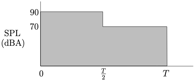
Example 1
Determine the equivalent sound level  for the period if the sound pressure level varies as shown below.
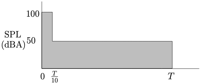
Example 2
Determine the equivalent sound level for the period if the sound pressure level varies as shown below.
Example 3
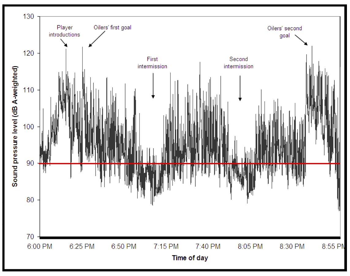
During the 2006 Edmonton Oiler’s run to the Stanley Cup finals, Rexall Place was described as “loud”. For game #3 of the finals against the Carolina Hurricanes, a local audiologist had a colleague who was attending the game wear a data–logging noise dosimeter which measured the noise level near the wearer’s ear every second. The game lasted approximately 3 hours. The results of the measurements are shown below, with some moments of interest indicated.
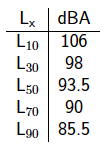
Levels
One means of quantifying this information is to use levels, which indicate the sound pressure level(dBA) that is exceeded percent of the time. The following table shows certain values for the sound pressure levels for game #3.
 Levels
Another method to quantify this data is to use the equivalent sound level LEQ which is the equivalent steady state sound pressure level that contains the same acoustic energy as the actual fluctuating values over a given period of time,

The data points shown in the figure are actually LEQ values based on one second time periods, calculated every second. For the entire game, the equivalent sound pressure level was  dBA based on the duration of the game.
Some Interesting Facts…
- L
 = 134.7 dBA
This is the maximum instantaneous sound pressure level (A-weighted) that occurred during the game. This is significantly higher than any data point shown in the figure, which are based LEQ values (a form of averaging) over each one second period. - L
 = 76.5 dBA
Similar to L, but represents the minimum sound pressure level that occurred. - 6 minutes
If this was a workplace, 6 minutes is the maximum time that you would be permitted to work in this environment without hearing protection based on current Occupational Health and Safety guidelines.
In fact even during the intermissions, which had the lowest sound pressure levels, the noise levels were such that if this was an 8hr/day work environment hearing protection would be required by law (85 dBA for 8 hours is generally considered to be the maximum allowable daily noise dose).