Forced Vibrations of Damped Single Degree of Freedom Systems: Damped Spring Mass System
We have so far considered harmonic forcing functions acting on undamped systems. We will now extend our analysis to include systems which include viscous damping. We will still limit our analysis to harmonic forcing functions of the form 
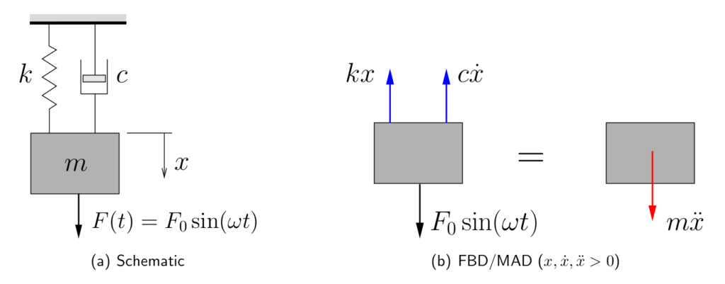
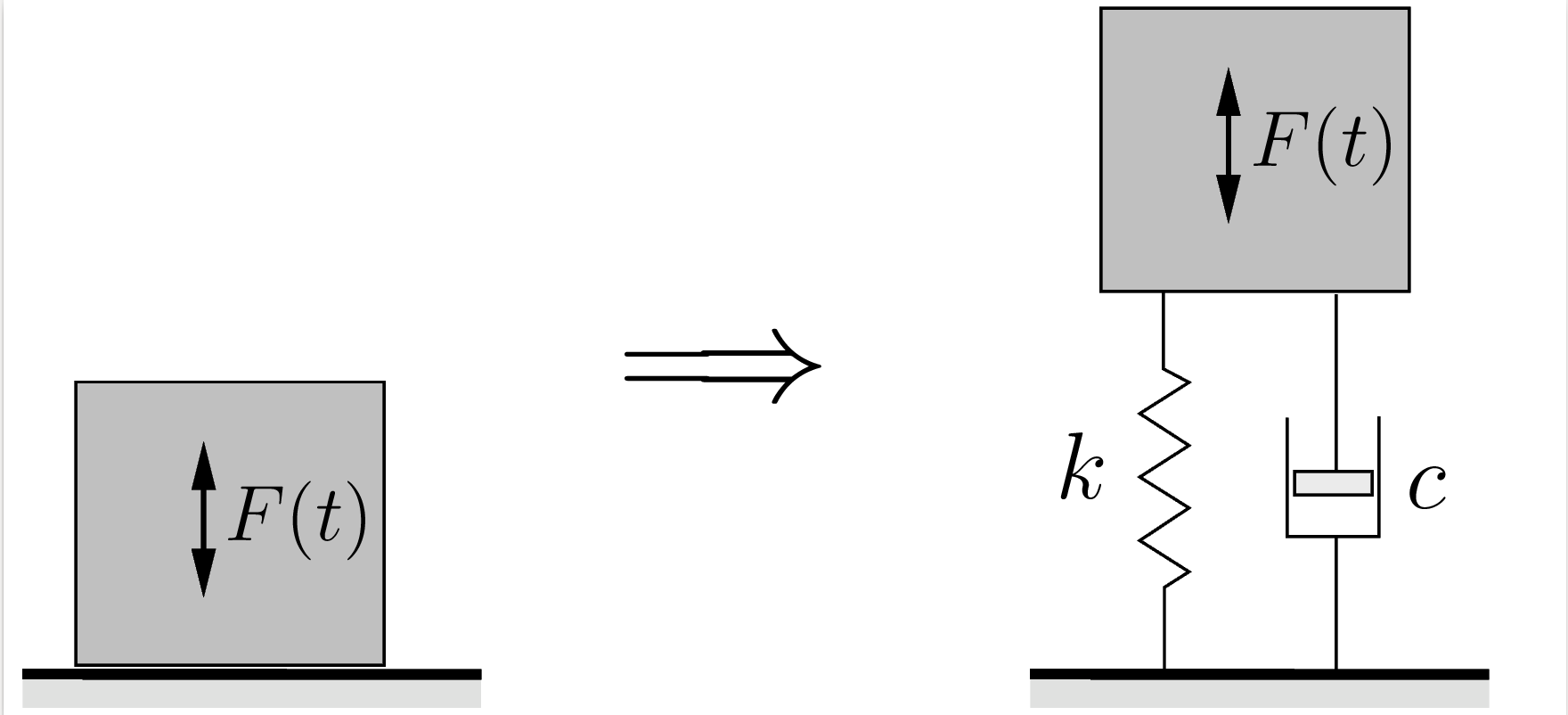
Consider a damped spring-mass system subjected to a harmonic forcing function as shown in Figure 5.1(a). The FBD/MAD for this system is shown in Figure 5.1(b) where  is once again the displacement from the static equilibrium position. Applying Newton’s Laws we obtain
![\[+\!\!\downarrow\sum F = ma:\qquad F_0 \sin(\omega t) -kx -c \dot{x} = m \ddot{x}\]](https://engcourses-uofa.ca/wp-content/ql-cache/quicklatex.com-eadd3881a24c8ab22de14ead9ea9fff6_l3.png "Rendered by QuickLaTeX.com")
or
(5.1) ![\[m \ddot{x} + c\dot{x} + kx = F_0 \sin(\omega t) \]](https://engcourses-uofa.ca/wp-content/ql-cache/quicklatex.com-e158386201ba9f0e46a058d4b609d4a4_l3.png "Rendered by QuickLaTeX.com")
Once again, the response  will be composed of a homogeneous solution (the transient response) and a particular solution (the steady state response) as
(5.2) ![\[x(t) = x_H(t) + x_P(t)\]](https://engcourses-uofa.ca/wp-content/ql-cache/quicklatex.com-9d4e8a1f696e0a1d03b5a9bb843ab54a_l3.png "Rendered by QuickLaTeX.com")
We have previously found the homogeneous solution. For example, in the underdamped situation the homogeneous solution  is given in equation (3.11) as
(5.3) ![\[x_H(t) = e^{-\zeta p t} \Bigl[ A \sin(\sqrt{1-\zeta^2}pt) + B \cos(\sqrt{1-\zeta^2}pt) \Bigr]\]](https://engcourses-uofa.ca/wp-content/ql-cache/quicklatex.com-42190ecaf0ddf3d044f784d60497e91a_l3.png "Rendered by QuickLaTeX.com")
where  and
and  are arbitrary constants. To find the particular solution to equation (5.1), we will
assume a solution of the form
(5.4) ![\[x_P(t) =\phantom{-} \mathbb{X} \sin\left(\omega t - \phi\right)\]](https://engcourses-uofa.ca/wp-content/ql-cache/quicklatex.com-6eff60a02271340c62243c97ed608d04_l3.png "Rendered by QuickLaTeX.com")
so that

Substituting these into the equation of motion gives
(5.5) ![\[m \Bigl[ -\mathbb{X} \, \omega^2\sin\left(\omega t - \phi\right) \Bigr]+c \Bigl[ \mathbb{X} \, \omega \cos\left(\omega t - \phi\right) \Bigr]+k \Bigl[ \mathbb{X} \, \sin\left(\omega t - \phi\right) \Bigr] = F_0 \sin (\omega t)\]](https://engcourses-uofa.ca/wp-content/ql-cache/quicklatex.com-a45685e5f438e8787e71c99967e464ee_l3.png "Rendered by QuickLaTeX.com")
Using the identities

results in
![\[\mathbb{X} \bigl(k-m\omega^2\bigr) \Bigl[ \sin \omega t \cos \phi - \cos \omega t \sin \phi \Bigr] +c \mathbb{X} \omega \Bigl[ \cos \omega t \cos \phi + \sin \omega t \sin \phi \Bigr] = F_0 \sin \omega t\]](https://engcourses-uofa.ca/wp-content/ql-cache/quicklatex.com-adc2a67577b667e2f69011f4986724e5_l3.png "Rendered by QuickLaTeX.com")
or, collecting the  and
and  terms,
![\[\mathbb{X} \Bigl[ \bigl(k-m\omega^2\bigr) \cos \phi + c \omega \sin \phi \Bigr] \sin \omega t -\mathbb{X} \Bigl[ \bigl(k-m\omega^2\bigr) \sin \phi - c \omega \cos \phi \Bigr] \cos \omega t = F_0 \sin \omega t\]](https://engcourses-uofa.ca/wp-content/ql-cache/quicklatex.com-41661a1c76871fb738211f9c835311ff_l3.png "Rendered by QuickLaTeX.com")
Comparing the left and right hand sides leads to two equations
(5.6a) ![\[ \mathbb{X} \Bigl[ \bigl(k-m\omega^2\bigr) \cos \phi + c \omega \sin \phi \Bigr] = F_0\]](https://engcourses-uofa.ca/wp-content/ql-cache/quicklatex.com-273aa65ed8b5e6f3ed76b680a1887aee_l3.png "Rendered by QuickLaTeX.com")
(5.6b) ![\[ \mathbb{X} \Bigl[ \bigl(k-m\omega^2\bigr) \sin \phi - c \omega \cos \phi \Bigr] = 0\]](https://engcourses-uofa.ca/wp-content/ql-cache/quicklatex.com-01ea9c198e10a85f3417150c7c3cadd0_l3.png "Rendered by QuickLaTeX.com")
From (5.6b) we see that
![\[\bigl(k-m\omega^2\bigr) \sin \phi = c \omega \cos \phi\]](https://engcourses-uofa.ca/wp-content/ql-cache/quicklatex.com-3030b5b1bff512f2ede4112f0ec7d47f_l3.png "Rendered by QuickLaTeX.com")
so that
![\[\frac{\sin \phi}{\cos \phi} = \tan \phi = \frac{c \omega}{k-m\omega^2}\]](https://engcourses-uofa.ca/wp-content/ql-cache/quicklatex.com-9fbf18a2fc8c5a4f5a809bfb60ddb16e_l3.png "Rendered by QuickLaTeX.com")
or
(5.7) ![\[\boxed{\phi = \tan^{-1} \biggl[ \frac{c \omega}{k-m\omega^2} \biggr]} \]](https://engcourses-uofa.ca/wp-content/ql-cache/quicklatex.com-639491b484d95a14570eaf8b97aeb147_l3.png "Rendered by QuickLaTeX.com")
 (
( gives
gives ![\[\mathbb X \bigl(k-m\omega^2\bigr) \bigr(\cancelto{1}{\cos^2 \phi + \sin^2 \phi}\bigr) = F_0 \cos \phi\]](https://engcourses-uofa.ca/wp-content/ql-cache/quicklatex.com-ecaf782e96ef958ba9e4e6b32ffe22aa_l3.png "Rendered by QuickLaTeX.com")
(5.8a) ![\[\mathbb{X} \bigl(k-m\omega^2\bigr) = F_0 \cos \phi\]](https://engcourses-uofa.ca/wp-content/ql-cache/quicklatex.com-0ba71d220d3223d62c0751a824df4d90_l3.png "Rendered by QuickLaTeX.com")
 gives
gives ![\[\mathbb{X} c \omega \bigr(\cancelto{1}{\sin^2 \phi + \cos^2 \phi} \bigr) = F_0 \sin \phi\]](https://engcourses-uofa.ca/wp-content/ql-cache/quicklatex.com-2899f1d17ecf2169122d488c9c6809b3_l3.png "Rendered by QuickLaTeX.com")
(5.8b) ![\[\mathbb{X} c \omega = F_0 \sin \phi\]](https://engcourses-uofa.ca/wp-content/ql-cache/quicklatex.com-e559877d206e360f9ce24cb1bb4bc57e_l3.png "Rendered by QuickLaTeX.com")
Squaring each of (5.8a) and (5.8b) and adding the results leads to
![\[F_0^2 = \mathbb{X}^2 \Bigl[ \bigl(k-m\omega^2\bigr)^2 + \bigl(c \omega \bigr)^2 \Bigr]\]](https://engcourses-uofa.ca/wp-content/ql-cache/quicklatex.com-5938518197a0b1dd27ef8943bff6c7fb_l3.png "Rendered by QuickLaTeX.com")
or
(5.9) ![\[\boxed{\mathbb{X} = \frac{F_0}{\sqrt{\bigl(k-m\omega^2\bigr)^2 + \bigl(c \omega \bigr)^2}}}\]](https://engcourses-uofa.ca/wp-content/ql-cache/quicklatex.com-8c66b4a8ec7457b1ccc8e0ed9dd5a08e_l3.png "Rendered by QuickLaTeX.com")
Therefore, the particular solution (5.4) for this problem is
(5.10) ![\[x_P(t) = \frac{F_0}{\sqrt{\bigl(k-m\omega^2\bigr)^2 + \bigl(c \omega \bigr)^2}} \sin (\omega t - \phi)\]](https://engcourses-uofa.ca/wp-content/ql-cache/quicklatex.com-44d42fb8d44c609461989a7baf82b636_l3.png "Rendered by QuickLaTeX.com")
where  is given by equation (5.7). The total solution (for the underdamped case) is
![\[x(t) = e^{-\zeta p t} \Bigl[ A \sin\left(\sqrt{1-\zeta^2}pt\right) + B\cos\left(\sqrt{1-\zeta^2}pt\right) \Bigr] + \frac{F_0}{\sqrt{\bigl(k-m\omega^2\bigr)^2 + \bigl(c \omega \bigr)^2}} \sin(\omega t - \phi)\]](https://engcourses-uofa.ca/wp-content/ql-cache/quicklatex.com-e98f61305474d1a66c9d20555e937bac_l3.png "Rendered by QuickLaTeX.com")
In many cases we are often primarily interested in the long term steady state response of a system. Since the transient response will eventually damp out as we have seen, we will often ignore the transient part and consider the solution to be simply given by the steady state response as
(5.11) ![\[x(t) = \frac{F_0}{\sqrt{\bigl(k-m\omega^2\bigr)^2 + \bigl(c \omega \bigr)^2}} \sin (\omega t - \phi)\]](https://engcourses-uofa.ca/wp-content/ql-cache/quicklatex.com-a2fbd32f69bd5dc902920b7f9db57b9d_l3.png "Rendered by QuickLaTeX.com")
Note that this can be rewritten as
(5.12) ![\[x(t) = \frac{\dfrac{F_0}{k}}{\sqrt{\Bigl(1-\dfrac{m}{k}\omega^2\Bigr)^2 + \Bigl(\dfrac{c \omega}{k} \Bigr)^2}} \sin (\omega t - \phi)\]](https://engcourses-uofa.ca/wp-content/ql-cache/quicklatex.com-b5ea1adceb2956265203e5b1e8b2b1cb_l3.png "Rendered by QuickLaTeX.com")
However, as we have already discussed,
![\[\frac{F_0}{k} = \ensuremath{\delta_{\mathrm{ST}}},\qquad \frac{m}{k} = \frac{1}{\ensuremath{p}^2},\]](https://engcourses-uofa.ca/wp-content/ql-cache/quicklatex.com-4f80e36f8bf8e7f264e913a7a1ba1a01_l3.png "Rendered by QuickLaTeX.com")
and
![\[\frac{c\omega}{k} = c \, \left(\frac{2 m\ensuremath{p}}{c_\mathrm{C}}\right) \, \frac{\omega}{k}= 2 \, \cancelto{\zeta}{\frac{c}{c_\mathrm{C}}} \, \cancelto{\frac{1}{\ensuremath{p}^2}}{\frac{m}{k}} \, \ensuremath{p} \omega= 2 \zeta\frac{\omega}{\ensuremath{p}}\]](https://engcourses-uofa.ca/wp-content/ql-cache/quicklatex.com-46cf063f0f45ceef025f1ad051e48eff_l3.png "Rendered by QuickLaTeX.com")
As a result, (5.12) becomes
(5.13) ![\[x(t) = \underbrace{\frac{\ensuremath{\delta_{\mathrm{ST}}}}{\ensuremath{\sqrt{\left[1- \left(\ensuremath{\frac{\omega}{\ensuremath{p}}}\right)^2\right]^2 + \Bigl[2 \zeta \ensuremath{\frac{\omega}{\ensuremath{p}}} \Bigr]^2}}}}_{\text{Amplitude }\mathbb{X}} \, \sin (\omega t - \phi)\]](https://engcourses-uofa.ca/wp-content/ql-cache/quicklatex.com-0707a2819724b5f9c429729f864bcd41_l3.png "Rendered by QuickLaTeX.com")
Here we can see that the amplitude of the response is given by
![\[\mathbb{X} = \ensuremath{\delta_{\mathrm{ST}}} \frac{1}{\ensuremath{\sqrt{\left[1-\left(\ensuremath{\frac{\omega}{\ensuremath{p}}}\right)^2\right]^2 + \Bigl[2 \zeta \ensuremath{\frac{\omega}{\ensuremath{p}}} \Bigr]^2}}}\]](https://engcourses-uofa.ca/wp-content/ql-cache/quicklatex.com-07d55e7bd293690fe053b4a8da90dc0a_l3.png "Rendered by QuickLaTeX.com")
or
(5.14) ![\[\boxed{\frac{\mathbb{X}}{\ensuremath{\delta_{\mathrm{ST}}}} = \frac{1}{\ensuremath{\sqrt{\left[1-\left(\ensuremath{\frac{\omega}{\ensuremath{p}}}\right)^2\right]^2 + \Bigl[2 \zeta \ensuremath{\frac{\omega}{\ensuremath{p}}} \Bigr]^2}}}}\]](https://engcourses-uofa.ca/wp-content/ql-cache/quicklatex.com-e6c996b8c515081c07f0d593aea2e9aa_l3.png "Rendered by QuickLaTeX.com")
which represents the dynamic magnification factor in the damped situation. Similarly, since
![\[\frac{c\omega}{k-m\omega^2} = \frac{\dfrac{c \omega}{k}}{1-\dfrac{m}{k} \omega^2} =\dfrac{2 \zeta \ensuremath{\dfrac{\omega}{\ensuremath{p}}}}{1-\ensuremath{\dfrac{\omega}{\ensuremath{p}}}^2}\]](https://engcourses-uofa.ca/wp-content/ql-cache/quicklatex.com-76e8c2395909d7cf8fa0b399834e68da_l3.png "Rendered by QuickLaTeX.com")
equation (5.7) can be written as
(5.15) ![\[\boxed{\phi = \tan^{-1} \left[ \frac{2 \zeta \ensuremath{\frac{\omega}{\ensuremath{p}}}}{1-\left(\ensuremath{\frac{\omega}{\ensuremath{p}}}\right)^2} \right]}\]](https://engcourses-uofa.ca/wp-content/ql-cache/quicklatex.com-dbcfea291b483fbe213fe7770d91f1d4_l3.png "Rendered by QuickLaTeX.com")
Equations (5.14) and (5.15) are illustrated in Figures 5.2(a) and (b) respectively.
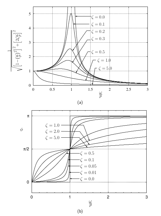
(a) In the limiting case where  , these results are the same as those obtained in the undamped case.

(b) At very low frequency ratios,  , the amplitude of the motion is approximately the static deflection.
(c) At very high frequency ratios,  , the amplitude of the response is significantly less than the static deflection.
(d) In both (b) and (c) above, damping has very little effect. Therefore at these extremes, it is often appropriate to use the results for an undamped system (simply because they are easier to use).
(e) Between these two extremes, and particularly near resonance, damping has the effect of limiting the amplitude of vibration. At resonance an infinite amplitude will never be reached and a steady state value can be obtained.
(f) When the system is damped, there is no sudden transition from in phase to completely out of phase. The response is always somewhat out of phase with the forcing function (we usually say the response lags the forcing function by the phase angle).
(g) At resonance, the response lags the forcing function by  radians, regardless of the amount of damping present.
Graphic Representation
Reconsider the response of the system in equation (5.5)
![\[m \Bigl[ -\mathbb{X} \omega^2\sin (\omega t - \phi) \Bigr]+c \Bigl[ \mathbb{X} \omega \cos (\omega t - \phi) \Bigr]+k \Bigl[ \mathbb{X} \sin (\omega t - \phi) \Bigr] = F_0 \sin \omega t,\]](https://engcourses-uofa.ca/wp-content/ql-cache/quicklatex.com-4e12f5cc13f2189956a5849a615083a2_l3.png "Rendered by QuickLaTeX.com")
and rearrange the results slightly as
(5.16) ![\[\underbrace{F_0 \sin \omega t\rule[-3mm]{0pt}{0pt}}_{\text{Disturbing Force}}- \underbrace{k \Bigl[ \mathbb{X} \sin (\omega t - \phi) \Bigr]}_{\text{Spring Force}}- \underbrace{c \Bigl[ \mathbb{X} \omega \cos (\omega t - \phi) \Bigr]}_{\text{Damping Force}}+ \underbrace{m \Bigl[ \mathbb{X} \omega^2\sin (\omega t - \phi) \Bigr]}_{\text{``Inertia'' Force}}= 0\]](https://engcourses-uofa.ca/wp-content/ql-cache/quicklatex.com-636a528a089729db3fe684af78231b2e_l3.png "Rendered by QuickLaTeX.com")
We can interpret each of the terms in this equation as the vertical component of a vector rotating CCW about the origin at a rate of  rad/s as shown in Figure 5.3 below.
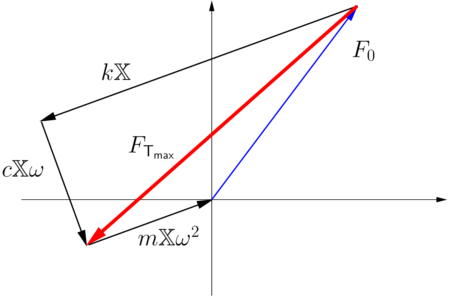
However, from (5.16) we see that the sum of these components must be zero. It is therefore convenient to add these terms vectorially so that the resulting polygon closes as in Figure 5.4.
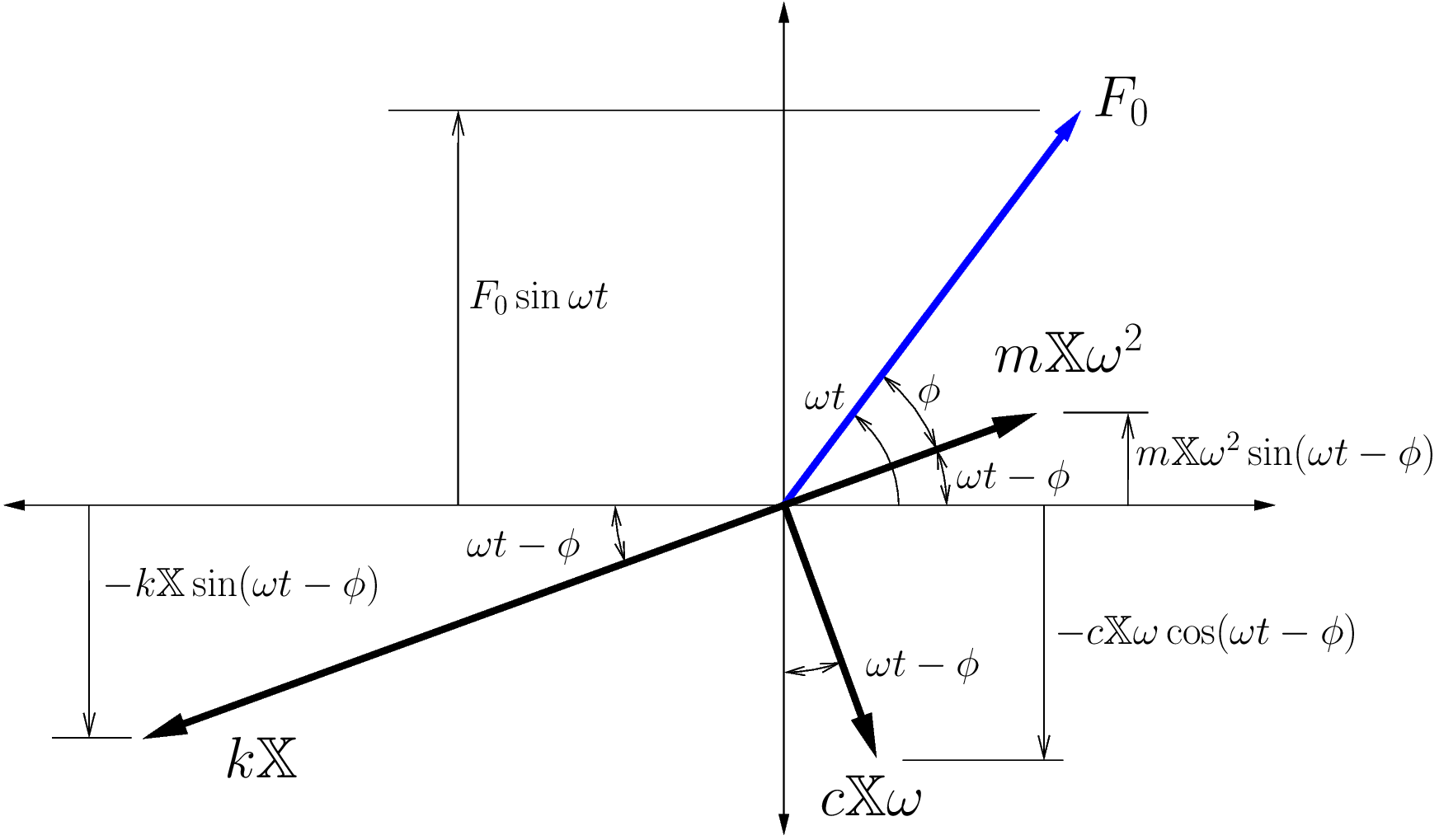
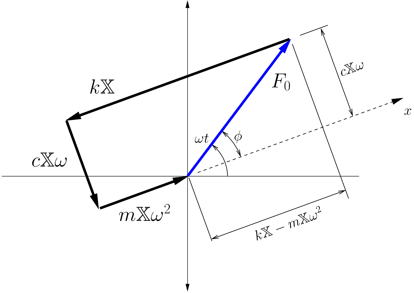
From this figure we can see clearly that
![\[F_0^2 = \Bigl[ k \mathbb{X} - m \mathbb{X} \omega^2 \Bigr]^2 + \Bigl[ c \mathbb{X} \omega \Bigr]^2 \qquad \text{and}\qquad\tan \phi = \frac{c \mathbb{X} \omega}{k \mathbb{X} - m \mathbb{X} \omega^2}\]](https://engcourses-uofa.ca/wp-content/ql-cache/quicklatex.com-6a96be70c99f1219066be945c5c6d2d6_l3.png "Rendered by QuickLaTeX.com")
which leads directly to
![\[\mathbb{X} = \frac{F_0}{\sqrt{\bigl(k-m\omega^2\bigr)^2 + \bigl(c \omega \bigr)^2}}\]](https://engcourses-uofa.ca/wp-content/ql-cache/quicklatex.com-e67d934b200e4aa0a917e15e7a356268_l3.png "Rendered by QuickLaTeX.com")
and
![\[\phi = \tan^{-1} \Bigl( \frac{c \omega}{k-m\omega^2} \Bigr)\]](https://engcourses-uofa.ca/wp-content/ql-cache/quicklatex.com-5fb8b904dd6db922d2997cef32e39b34_l3.png "Rendered by QuickLaTeX.com")
which are the results obtained previously (but with less work involved here).
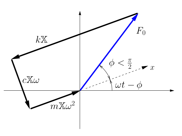
Using this representation, we can understand the effect of damping in each of the three situations
![\[\ensuremath{\frac{\omega}{\ensuremath{p}}} < 1,\qquad \ensuremath{\frac{\omega}{\ensuremath{p}}} = 1,\qquad \ensuremath{\frac{\omega}{\ensuremath{p}}} > 1.\]](https://engcourses-uofa.ca/wp-content/ql-cache/quicklatex.com-c38bc78d0432f0ad12876c0662bdb5e4_l3.png "Rendered by QuickLaTeX.com")

In this case, the  term is smaller than the
  term. As a result, the inertia force is smaller than the spring force. As a result, the phase angle (the angle by which the response lags the forcing function) is less than
  .
.

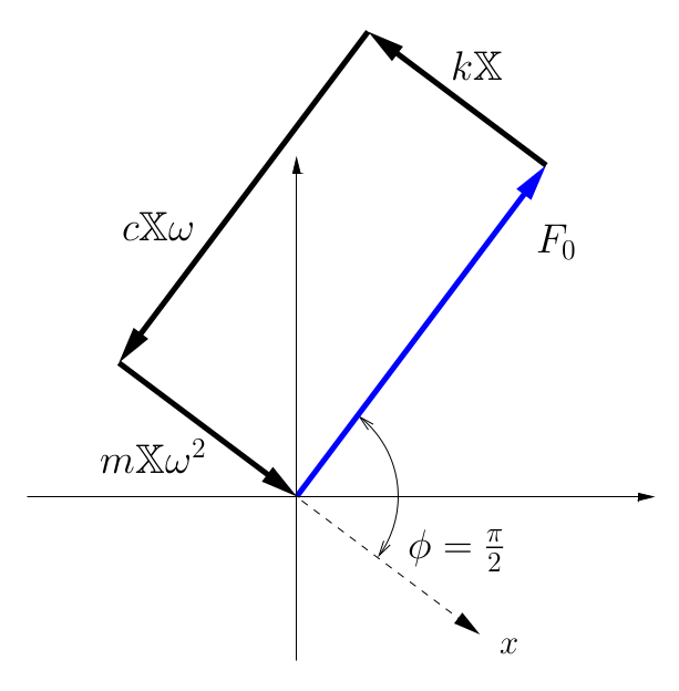
Here the inertia force exactly balances the spring force, while the disturbing force exactly balances the damping force. As a result, we see that the phase angle is always radians.

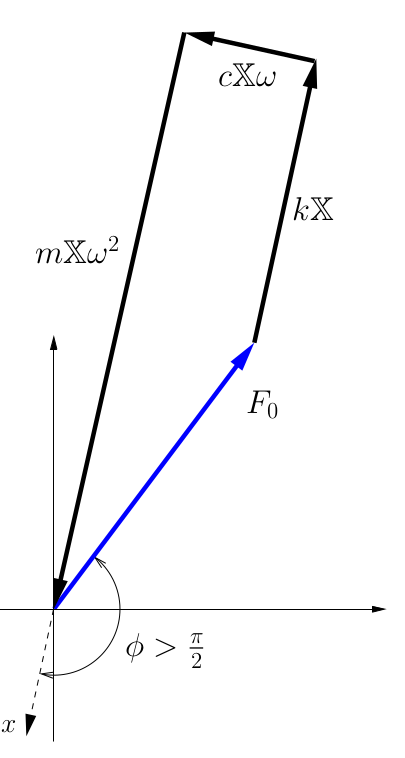
Here, the inertia forces are larger than the spring forces. The result is a larger phase angle, somewhere between and  radians.
The tool below demonstrates the rotating vector representation. In the tool  is the natural frequency
  . Change the parameters to see the effect on the vector schematic.
Transmissibility in Forced Damped Vibrations
The force transmitted between a machine and its supporting structure is an important consideration in the vibration isolation of machinery. Typically a machine is vibrating due to some internal disturbing force and we would like to isolate the supporting structure from these vibrations. (The reverse situation also applies.)
A typical situation is shown in Figure 5.5. The goal is often to reduce the maximum force transmitted to the supporting structure. When we previously considered the undamped situation, the only force transmitted to the support was through the spring. Now, however, force can be transmitted through both the spring and the damper. Further, we can not simply added these two forces as scalars because they do not reach their maximum values at the same time (i.e. they are not in phase). However, as we have seen these two forces are always 90 out of phase
![\[F_\text{S} = k x(t) = k \mathbb{X} \sin (\omega t - \phi),\qquad F_\text{C} = c \dot{x}(t) = c \mathbb{X} \omega \cos (\omega t - \phi)\]](https://engcourses-uofa.ca/wp-content/ql-cache/quicklatex.com-c782b68c453f542d615417d707440ca6_l3.png "Rendered by QuickLaTeX.com")
so the resulting magnitude of the sum of these two forces is
![\[F_{T_{max}} = \sqrt{\bigl( k \mathbb{X} \bigr)^2 + \bigl( c \mathbb{X} \omega\bigr)^2}\]](https://engcourses-uofa.ca/wp-content/ql-cache/quicklatex.com-83733d242493edfb7f1325df171ddd6a_l3.png "Rendered by QuickLaTeX.com")
or
(5.17) ![\[F_{T_{max}} = k \mathbb{X} \sqrt{1 + \Bigl( \frac{c \omega}{k}\Bigr)^2}\]](https://engcourses-uofa.ca/wp-content/ql-cache/quicklatex.com-b99cc829a8dc880542f8b1f83c0e8715_l3.png "Rendered by QuickLaTeX.com")
(This force can be seen schematically in the diagram in Figure 5.6 based on the graphical interpretation discussed earlier.) However, we have already determined the amplitude of the response in this situation (equation (5.9)) to be
or
(5.18) ![\[\mathbb{X} = \frac{\dfrac{F_0}{k}}{\sqrt{\Bigl[1-\dfrac{m}{k}\omega^2\Bigr]^2 +\Bigl[\dfrac{c \omega}{k} \Bigr]^2}}\]](https://engcourses-uofa.ca/wp-content/ql-cache/quicklatex.com-f7624e60298191d1ccd4794397f82b24_l3.png "Rendered by QuickLaTeX.com")
 transmitted to the supporting structure
Combining (5.17) and (5.18) gives
![\[\ensuremath{F_{T_{max}}}} = \cancel k \cdot\frac{\frac{F_0}{\cancel k}}{\sqrt{\Bigl[1-\frac{m}{k}\omega^2\Bigr]^2 +\Bigl[\frac{c \omega}{k} \Bigr]^2}}\cdot\sqrt{1 + \Bigl( \frac{c \omega}{k}\Bigr)^2}\]](https://engcourses-uofa.ca/wp-content/ql-cache/quicklatex.com-54930033721ead8c2c0e515f1310bfb9_l3.png "Rendered by QuickLaTeX.com")
or
![\[\frac{F_{T_{max}}}{F_0} = \frac{\sqrt{1 + \Bigl( \dfrac{c \omega}{k}\Bigr)^2}}{\sqrt{\Bigl[1-\dfrac{m}{k}\omega^2\Bigr]^2 +\Bigl[\dfrac{c \omega}{k} \Bigr]^2}}\]](https://engcourses-uofa.ca/wp-content/ql-cache/quicklatex.com-3c9bb7f7e5e8ecbe4a26a59262423bf8_l3.png "Rendered by QuickLaTeX.com")
Recalling that
![\[\frac{m}{k}\omega^2 = \Bigl(\ensuremath{\frac{\omega}{\ensuremath{p}}}\Bigr)^2 \qquad\text{and}\qquad\frac{c\omega}{k} = 2\zeta\ensuremath{\frac{\omega}{\ensuremath{p}}}\]](https://engcourses-uofa.ca/wp-content/ql-cache/quicklatex.com-ed61f84114762e5a7750b84e8a5a3eb6_l3.png "Rendered by QuickLaTeX.com")
we get the result
(5.19) ![\[\boxed{\ensuremath{TR} = \frac{F_{T_{max}}}{F_0} = \frac{\sqrt{1 + \Bigl( 2 \zeta \ensuremath{\dfrac{\omega}{\ensuremath{p}}} \Bigr)^2}}{\ensuremath{\sqrt{\left[1-\ensuremath{\left(\frac{\omega}{\ensuremath{p}}}\right)^2\right]^2 + \Bigl[2 \zeta \ensuremath{\frac{\omega}{\ensuremath{p}}} \Bigr]^2}}}}\]](https://engcourses-uofa.ca/wp-content/ql-cache/quicklatex.com-758e1c4e2aff2e78de98270ca22901c8_l3.png "Rendered by QuickLaTeX.com")
This is the transmissibility in the damped situation which represents the ratio of the maximum force transmitted to the supporting structure to the maximum disturbing force (which here is simply  ).
).
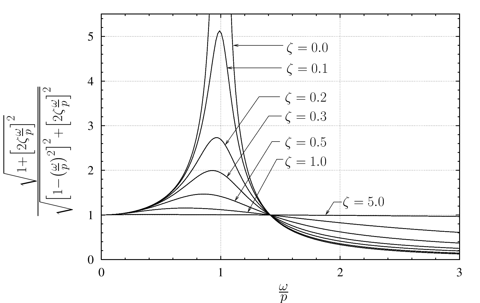
This relationship is illustrated in Figure 5.7. As this figure shows, the transmissibility is always greater than one if  . This means that more force is transmitted to the supporting structure than if the machine were rigidly attached to the structure. Near resonance, even small amounts of damping can significantly reduce the force transmitted to the structure.
For  , the force transmitted to the structure is less than the disturbing force. In this region, however, the addition of damping increases the transmissibility compared to the undamped situation. If a system is operating in this region, an undamped support offers better transmissibility characteristics than one with damping. However, some damping is often still desirable if the system must pass through resonance to reach its operating state.
EXAMPLE
A machine with a mass of 100 kg is supported on springs of total stiffness 700 kN/m and has an unbalanced rotating element which results in a disturbing force of 350 N at a speed of 3000 RPM. Assuming the system has a damping ratio of  , determine
- the amplitude of the motion due to the rotating imbalance,
- the transmissibility, and
- the maximum force transmitted to the supporting structure.
EXAMPLE
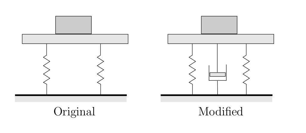
A vibrating system, together with its inertia base, is originally mounted on a set of springs. The operating frequency of the machine is 230 RPM. The system weighs 1000 N and has an effective spring modulus 4000 N/m. Shock absorbers are to be added to the system to reduce the transmissibility at resonance to 3. Additionally, the transmissibility at the normal operating speed should be kept below 0.2.
- Without damping, what is the transmissibility at the operating speed?
- Is it possible to pick a damper which satisfies the above conditions? If so, what range of values of the damping ratio (
 ) will satisfy these two conditions?
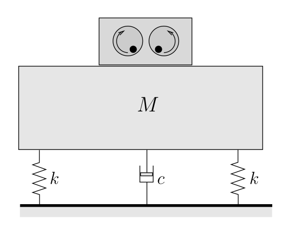
Forced Vibrations Due to a Rotating Imbalance
A common cause of forced vibrations in machinery is a rotating imbalance, shown schematically in Figure 5.8.
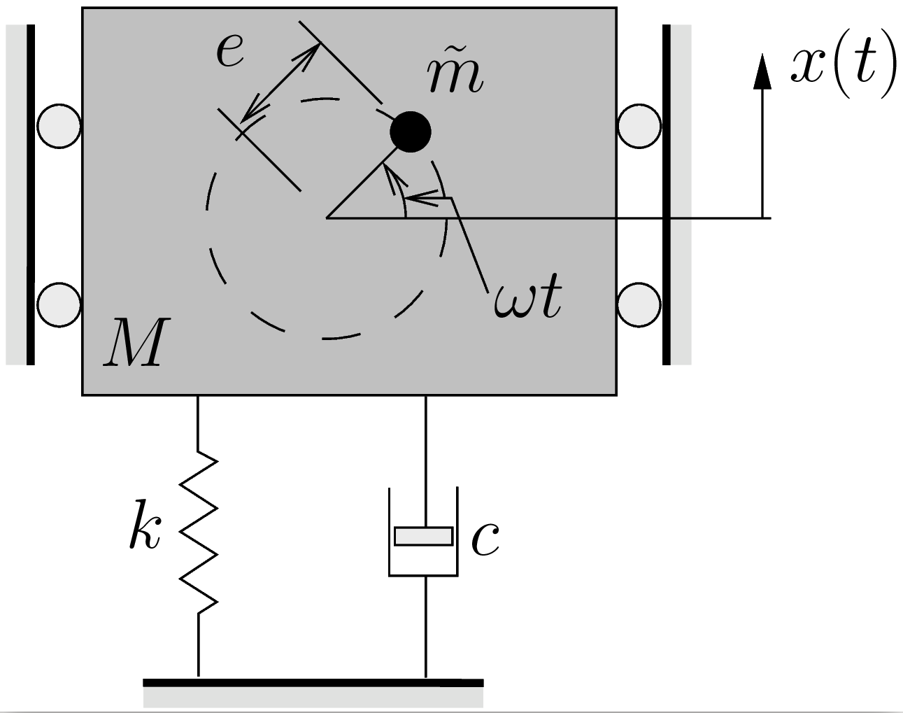
Here a machine with total mass  is constrained to move in a vertical direction.
  is a rotating mass (which is included in the total mass ) with eccentricity
  that is rotating at a constant speed . During the resulting motion the machine body (the part that is not the eccentric mass) vibrates vertically, with a position described by the cooordinate . The eccentric mass moves relative to the machine body, and its total vertical displacement is given by
  .
.
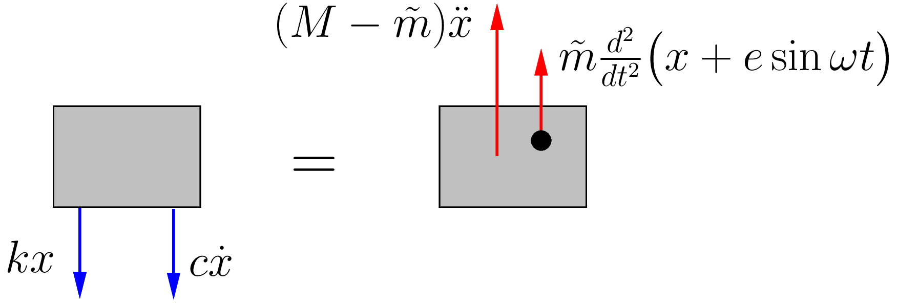
Figure 5.9 shows a FBD/MAD for this situtation. Applying Newton’s Laws in the vertical direction gives

(5.20) ![\[M \ddot{x} + c\dot{x} + k x = \underbrace{\ensuremath{\tilde{m} e \omega^2}\rule[-1mm]{0pt}{0pt}}_{F_0} \sin \omega t.\]](https://engcourses-uofa.ca/wp-content/ql-cache/quicklatex.com-e118d7f8866e9a188a0a8bc65657c479_l3.png "Rendered by QuickLaTeX.com")
This is the same equation of motion we obtained previously (equation (5.1)) with
![\[F_0 = \ensuremath{\tilde{m} e \omega^2}.\]](https://engcourses-uofa.ca/wp-content/ql-cache/quicklatex.com-390b4ad78060b319e4384396ff446dbc_l3.png "Rendered by QuickLaTeX.com")
As a result we know the solution to the steady response is
![\[x(t) = \mathbb{X} \sin (\omega t - \phi)\]](https://engcourses-uofa.ca/wp-content/ql-cache/quicklatex.com-7b273f22b30a047db7200e2ea0a6d835_l3.png "Rendered by QuickLaTeX.com")
where
(5.21) ![\[\mathbb{X} = \frac{\dfrac{\ensuremath{\tilde{m} e \omega^2}}{k}}{\ensuremath{\sqrt{\Bigl[1-\ensuremath{\Bigl(\dfrac{\omega}{\ensuremath{p}}\Bigr)}^2\Bigr]^2 + \Bigl[2 \zeta \ensuremath{\dfrac{\omega}{\ensuremath{p}}} \Bigr]^2}}}, \qquad\phi = \tan^{-1} \Biggl[ \frac{2 \zeta \ensuremath{\frac{\omega}{\ensuremath{p}}}}{1-\left(\ensuremath{\frac{\omega}{\ensuremath{p}}}\right)^2} \rule[-1cm]{0pt}{0pt}\Biggr]\]](https://engcourses-uofa.ca/wp-content/ql-cache/quicklatex.com-4c4e209e853576ea599b0d8b7fa78859_l3.png "Rendered by QuickLaTeX.com")
As discussed previously,
![\[\frac{\ensuremath{\tilde{m} e \omega^2}}{k} = \frac{\ensuremath{\tilde{m}} e}{M} \left(\ensuremath{\dfrac{\omega}{\ensuremath{p}}}\right)^2\]](https://engcourses-uofa.ca/wp-content/ql-cache/quicklatex.com-336bd00ca7fffa1bd699e7e7353512d5_l3.png "Rendered by QuickLaTeX.com")
so that equation (5.21) can be rearranged to give
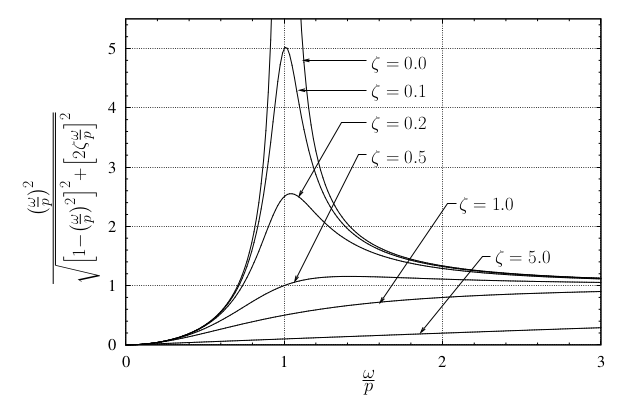
(5.22) ![\[\boxed{\frac{M\mathbb{X}}{\ensuremath{\tilde{m}} e} = \frac{\left(\ensuremath{\dfrac{\omega}{\ensuremath{p}}}\right)^2}{\ensuremath{\sqrt{\Bigl[1-\ensuremath{\Bigl(\dfrac{\omega}{\ensuremath{p}}\Bigr)}^2\Bigr]^2 + \Bigl[2 \zeta \ensuremath{\dfrac{\omega}{\ensuremath{p}}} \Bigr]^2}}}}\]](https://engcourses-uofa.ca/wp-content/ql-cache/quicklatex.com-8d9d59602d18f6f4300a8a1053bb3455_l3.png "Rendered by QuickLaTeX.com")
This result is shown in Figure 5.10 for a variety of damping ratios.
Note:
- At slow speeds
 , the disturbing force (
 ) is small so the response is correspondingly small.
 - At resonance (
 ) we can see that
![\[\frac{M\mathbb{X}}{\ensuremath{\tilde{m}} e} = \frac{1}{2\zeta}, %, \qquad\phi = \frac{\pi}{2}\]](https://engcourses-uofa.ca/wp-content/ql-cache/quicklatex.com-559b9af9d77601ca346b72f52f40ebe3_l3.png "Rendered by QuickLaTeX.com")
which illustrates that the steady state amplitude of the response at resonance is dependent on the amount of damping in the system. - At very high speeds,
 and the center of mass of the system remains approximately stationary as discussed for the undamped case.
 - As discussed previously, for an undamped system these results simplify to
![\[\frac{M\mathbb{X}}{\ensuremath{\tilde{m}} e} = \frac{\left(\ensuremath{\dfrac{\omega}{\ensuremath{p}}}\right)^2}{\ensuremath{\Bigl|1- \Bigl(\dfrac{\omega}{\ensuremath{p}}\Bigr)^2\Bigr|}}, \qquad \phi =\begin{cases}0,& \ensuremath{\dfrac{\omega}{\ensuremath{p}}} < 1, \\[6mm] \pi,& \ensuremath{\dfrac{\omega}{\ensuremath{p}}} > 1.\end{cases}\]](https://engcourses-uofa.ca/wp-content/ql-cache/quicklatex.com-ecce824222c83e829427e7a13e2c6819_l3.png "Rendered by QuickLaTeX.com")
EXAMPLE
A counter-rotating eccentric weight exciter is used to produce the forced oscillation of a spring and damper supported mass as shown below. By varying the rotation speed, a resonant amplitude of 0.60 cm was recorded. When the speed of rotation was increased considerably beyond the natural frequency, the amplitude appeared to approach a constant value of 0.08 cm.
Determine the damping ratio for the system.