Engineering at Alberta Courses » Coupling of Equations of Motion

Multiple Degree of Freedom Systems: Coupling of Equations of Motion

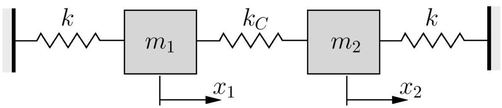
This image has an empty alt attribute; its file name is TDOF_Systems_Approx_Ex_002_Fig_a-eps-converted-to-page-001-1024x222.jpg — Figure 8.7: Simple two degree of freedom system

The simple two degree of freedom system we have been considering so far is shown in Figure (8.1), repeated here for convenience, for which the equations of motion were found to be

(8.20) $\begin{equation*}\label{eq:8.20}\begin{split}m \ddot{x}_1 + \bigl( k + k_C \bigr) x_1 - k_C x_2 &= 0 \\m \ddot{x}_2 -k_C x_1 + \bigl( k + k_C \bigr) x_2 &= 0\end{split}\end{equation*}$

As mentioned, these equations are coupled since both $x_1$ and $x_2$ appear in each of these equations. The implication with coupled equations is that they must be solved as a system. Neither of the equations can be solved individually.

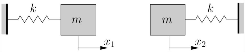
This image has an empty alt attribute; its file name is RealSimpletdofSystem-1024x220.jpg — Figure 8.8: Simpler two degree of freedom system

In contrast, consider the same system as above but with the central spring removed as shown in Figure 8.8. This is still a TDOF system as two coordinates are still required to completely specify the positions of the masses. The two equations of motion for this system are

(8.21) $\begin{equation*}\label{eq:8.21}\begin{split}m \ddot{x}_1 + k x_1 &= 0 \\m \ddot{x}_2 + k x_2 &= 0\end{split}\end{equation*}$

which can be seen to be uncoupled. The first equation is in terms of $x_1$ only while the second equation contains only $x_2$ . The solutions to these equations can be found immediately

(8.22) $\begin{equation*}\label{eq:8.22}\begin{split}x_1(t) &= A \sin{(p_1 t)} + B \cos{(p_1 t)} \\x_2(t) &= C \sin{(p_2 t)} + D \cos{(p_2 t)}\end{split}\end{equation*}$

where

$\begin{equation*}p_1 = \sqrt{\dfrac{k}{m}}, \qquad p_2 = \sqrt{\dfrac{k}{m}},\end{equation*}$

and $A, B, C$ and $D$ are arbitrary constants.

Note that in this case $p_1=p_2$ due to our choices for the system parameters. $p=p_2$ is not a general result for uncoupled systems.

As can be seen, uncoupled systems are significantly easier to solve that coupled ones. Review the effort required to obtain the solution to equations (8.20) and compare that to the effort required to obtain the solution to those in (8.21). The difference is apparent, and will become more significant as systems with more degrees of freedom are considered. It is hopefully clear from this that it is preferable to deal with uncoupled equations if possible.
Note that in matrix form, equations (8.20) and (8.21) are

(8.23) $\begin{equation*}\label{eq:8.23}\begin{bmatrix}m & 0 \\0 & m \\\end{bmatrix}\!\!\!\biggl\{\!\!\!\begin{array}{c}\ddot{x}_1 \\ \ddot{x}_2 \\\end{array}\!\!\!\biggr\}+\begin{bmatrix}k +k_C & -k_C \\-k_C & k+k_C \\\end{bmatrix}\!\!\!\biggl\{\!\!\!\begin{array}{c}x_1 \\ x_2 \\\end{array}\!\!\!\biggr\}=\biggl\{\!\!\!\begin{array}{c}0 \\ 0 \\\end{array}\!\!\!\biggr\}\end{equation*}$

and

(8.24) $\begin{equation*}\begin{bmatrix}m & 0 \\0 & m \\\end{bmatrix}\!\!\!\biggl\{\!\!\!\begin{array}{c}\ddot{x}_1 \\ \ddot{x}_2 \\\end{array}\!\!\!\biggr\}+\begin{bmatrix}k & 0 \\0 & k \\\end{bmatrix}\!\!\!\biggl\{\!\!\!\begin{array}{c}x_1 \\ x_2 \\\end{array}\!\!\!\biggr\}=\biggl\{\!\!\!\begin{array}{c}0 \\ 0 \\\end{array}\!\!\!\biggr\},\end{equation*}$

respectively. As can be seen, uncoupled equations correspond to diagonal matrices (both mass and stiffness matrices must be diagonal). Any off-diagonal term leads to a coupling of the equations. In equation (8.23) the off-diagonal terms occur in the stiffness matrix, which is referred to as static coupling. The situation in which the mass matrix contains off-diagonal is termed inertia coupling. It is possible for both type of coupling to be present at the same time.

Coupling and Coordinates

For the two degree of freedom system in Figure (8.7), the equations of motion are coupled as we have seen

$\begin{align*}m \ddot{x}_1 + \bigl( k + k_C \bigr) x_1 - k_C x_2 &= 0 \qquad (a) \\m \ddot{x}_2 - k_C x_1 + \bigl( k + k_C \bigr) x_2 &= 0 \qquad (b)\end{align*}$

Consider what happens however if we look at the sum and difference of these equations:

$\begin{align*}&(b)+(a):\qquad\qquad& m\ddot{x}_2 + m\ddot{x}_1 -{k_C} x_1 + \bigl( k + {k_C} \bigr) x_1+ \bigl( k + {k_C} \bigr) x_2 - {k_C} x_2 &= 0 \\&(b)-(a): & m\ddot{x}_2 - m\ddot{x}_1 -k_C x_1 - \bigl( k + k_C \bigr) x_1+ \bigl( k + k_C \bigr) x_2 + k_C x_2 &= 0\end{align*}$

$\begin{align*}m\left(\ddot{x}_2 + \ddot{x}_1\right) + k\left(x_2 + x_1\right) &= 0 \qquad (c) \\m\left(\ddot{x}_2 - \ddot{x}_1\right) + \left(k+2k_C\right)\left(x_2 - x_1\right) &= 0 \qquad (d)\end{align*}$

If we now define new coordinates $z_1$ and $z_2$ as

$\begin{align*}z_1 &= x_2 + x_1 \\z_2 &= x_2 - x_1\end{align*}$

$\begin{align*}m \ddot{z}_1 + k z_1 &= 0 \qquad (c*) \\m \ddot{z}_2 + \bigl( k + 2k_C \bigr) z_2 &= 0 \qquad (d*)\end{align*}$

which are now uncoupled. The solutions to these equations are therefore easy to write down as

$\begin{align*}z_1(t) &= \hat{A}\sin\left(p_1t\right) + \hat{B}\cos\left(p_1t\right) \qquad &(e) \\z_2(t) &= \hat{C}\sin\left(p_2t\right) + \hat{D}\cos\left(p_2t\right) \qquad &(f)\end{align*}$

where

(8.25) $\begin{equation*}p_1 = \sqrt{\frac{k}{m}}, \qquad p_2 = \sqrt{\frac{k+2k_C}{m}}\end{equation*}$

and $\hat{A}$ , $\hat{B}$ , $\hat{C}$ , and $\hat{D}$ are the arbitrary constants. Note that we get the same natural frequencies using this representation. Further, $x_1(t)$ and $x_2(t)$ can be found from $z_1(t)$ and $z_2(t)$ as

$\begin{align*}x_1(t) &= \frac{z_1(t) - z_2(t)}{2} \\x_2(t) &= \frac{z_1(t) + z_2(t)}{2}\end{align*}$

so that

$\begin{align*}\frac{(e)-(f)}{2} & \qquad x(t) &= \frac{\hat{A}}{2}\sin\left(p_1t\right) + \frac{\hat{B}}{2}\cos\left(p_1t\right) - \frac{\hat{C}}{2}\sin\left(p_2t\right) - \frac{\hat{D}}{2}\cos\left(p_2t\right) \\\frac{(e)+(f)}{2} & \qquad x(t) &= \frac{\hat{A}}{2}\sin\left(p_1t\right) + \frac{\hat{B}}{2}\cos\left(p_1t\right) + \frac{\hat{C}}{2}\sin\left(p_2t\right) + \frac{\hat{D}}{2}\cos\left(p_2t\right) \\\end{align*}$

$\begin{align*}x_1(t) &= A\sin\left(p_1t\right) + B\cos\left(p_1t\right) + C\sin\left(p_2t\right) + D\cos\left(p_2t\right) \\x_2(t) &= A\sin\left(p_1t\right) + B\cos\left(p_1t\right) - C\sin\left(p_2t\right) - D\cos\left(p_2t\right)\end{align*}$

where

$A = \frac{\hat{A}}{2}, \quad B = \frac{\hat{B}}{2}, \quad C = -\frac{\hat{C}}{2}, \quad D = -\frac{\hat{D}}{2}$

These can also be written as

$\begin{Bmatrix} x_1(t) \\ x_2(t) \end{Bmatrix} = \begin{Bmatrix} 1 \\ 1 \end{Bmatrix}\bigg[A\sin\left(p_1t\right) + B\cos\left(p_1t\right)\bigg]+ \begin{Bmatrix} 1 \\ -1 \end{Bmatrix}\bigg[C\sin\left(p_2t\right) + D\cos\left(p_2t\right)\bigg]$

which is exactly the same solution determined previously for this system in (8.15). Here we found the solution using only uncoupled equations in terms of the “coordinates” $x_2+x_1$ and $x_2-x_1$ . The important point of this exercise is to recognize that

Coupling is not a property of the system. Rather coupling is a consequence of the choice of coordinates used to describe the system.

Relationship to Mode Shapes
In the linear systems we have been discussing it is (almost) always possible to find a set of coordinates which uncouples the equations of motion. That is essentially what the mode shapes represent: linear combinations of the chosen coordinates that will uncouple the equations of motion:

$\begin{equation*}\underbrace{\biggl\{\!\!\!\begin{array}{r}1 \\ 1 \\\end{array}\!\!\!\biggr\} \Longrightarrow x_2 + x_1}_{\text{First Mode}}, \qquad\underbrace{\biggl\{\!\!\!\begin{array}{r}1 \\ -1 \\\end{array}\!\!\!\biggr\} \Longrightarrow -x_2 + x_1}_{\text{Second Mode}} \text{ or equivalently } x_2 - x_1.\end{equation*}$

In the current system, which is relatively simple, we were able to “guess” that the uncoupled coordinates would be $x_2 + x_1$ and $x_2-x_1$ . In general guessing like this is not very feasible. It was done here only to illustrate the concepts involved. For a general vibration problem, the uncoupled coordinates (i.e. mode shapes) can be found by following the procedure outlined earlier. This will work for (almost) all multiple degree of freedom systems.

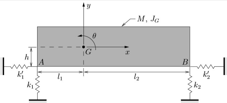
EXAMPLE

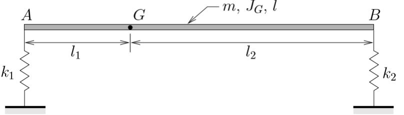
A rigid beam (mass $m$ , length $l$ , centroidal moment of inertia $J_G$ ) is supported by springs at its ends as shown. Determine the equations of motion, natural frequencies and mode shapes for this system.

This image has an empty alt attribute; its file name is Ex4a-8.jpg

Solve this problem using two different sets of coordinates:
(I) $x_1$ and $x_2$ ,
(II) $x_G$ and $\theta$ ,
as illustrated below.

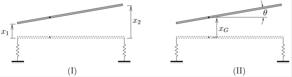
Be sure to identify any nodes in each mode shape.

EXAMPLE

An asymmetric machine mounting is supported by both vertical and horizontal springs as shown below.

(a) Using the coordinates $x$ , $y$ , and $\theta$ as illustrated, determine the equations of motion for this system.
(b) Explain how the equations of motion and mode shapes change in each of the following special cases:
(i) $k_2 \, l_2 = k_1 \, l_1$ ,
(ii) $h=0$ ,
(iii) $k_2 \, l_2 = k_1 \, l_1$ and $h=0$ .

EXAMPLE

The two degree of freedom system shown consists of a wheel (with mass $m_1$ and centroidal moment of inertia $J_O = m_1 r^2$ ) which rolls without slipping and a bar (with mass $m_2$ and centroidal moment of inertia $J_G = \frac{1}{3} m_2 L^2$ ) connected by three springs each of stiffness $k$ .

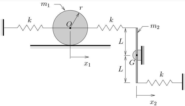
(a) Using the coordinates $x_1$ (the horizontal position of the center of the wheel) and $x_2$ (the horizontal position of the lower end of the bar) show that if $m_1 = m$ and $m_2 = 3m$ , the equations of motion for this system become

$\begin{equation*}\begin{bmatrix}2 m & 0 \\0 & m \\\end{bmatrix}\biggl\{\begin{array}{c}\ddot{x}_1 \\ \ddot{x}_2 \\\end{array}\biggr\}+\begin{bmatrix}2 k & k \\k & 2k \\\end{bmatrix}\biggl\{\begin{array}{c}x_1 \\ x_2 \\\end{array}\biggr\}=\biggl\{\begin{array}{c}0 \\ 0 \\\end{array}\biggr\}\end{equation*}$

(b) Determine the natural frequencies and mode shapes for this system.

Open Educational Resources

Multiple Degree of Freedom Systems: Coupling of Equations of Motion

Coupling and Coordinates

EXAMPLE

EXAMPLE

EXAMPLE

Leave a Reply Cancel reply