Engineering at Alberta Courses » Free Vibrations of a Damped Spring

Damped Free Vibrations of Single Degree of Freedom Systems: Free Vibrations of a Damped Spring–Mass System

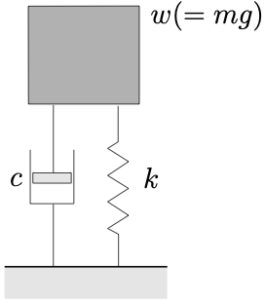
We now consider the simplest damped vibrating system shown in Figure 3.1. This is similar to the system considered previously but a linear damper has been added. We will use $x$ , the displacement from the equilibrium position, as the coordinate. A FBD for this system is shown as well.

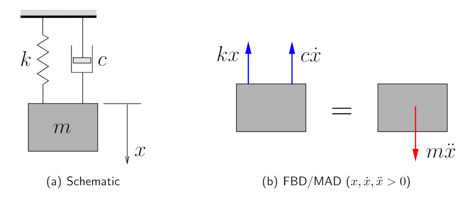
Figure 3.1 : Damped spring-mass system and FBD

Applying Newton’s Laws we get

$+\!\!\downarrow\sum F = ma\qquad\rightarrow\qquad -kx -c\dot{x} = m \ddot{x}$

(3.1) $\begin{equation*}\boxed{m \ddot{x} + c\dot{x} + kx = 0}\end{equation*}$

This governing equation of motion for this system is a linear, second order differential equation with constant coefficients. To solve it, we look for solutions of the form

$x(t) = C e^{st}$

so that

$\dot{x}(t) = C s e^{st}$

$\ddot{x}(t) = C s^2 e^{st}$

Substituting these into equation 3.1 results in

$m\left[\cancel{C} s^2 \cancel{e^{st}}\right] + c\left[\cancel{C} s \cancel{e^{st}}\right] + k\left[\cancel{C e^{st}}\right] = 0$

(3.2) $\begin{equation*}m s^2 + c s + k = 0\end{equation*}$

Equation 3.2 is the characteristic equation that is used to determine the values of $s$ . Solving equation 3.2 for $s$ gives

$s_{1,2} = \frac{-c \pm \sqrt{c^2 - 4 m k}}{2m} \notag$

(3.3) $\begin{equation*}s_{1,2} = \frac{-c}{2m} \pm \sqrt{\Bigl(\frac{c}{2m}\Bigr)^2 - \frac{k}{m}}\end{equation*}$

Each of the roots $s_1$ and $s_2$ provides a solution to equation 3.1

$x_1(t) = C_1 e^{s_1 t} \qquad x_2(t) = C_2 e^{s_2 t}$

and the total solution to equation 3.1 is a linear combination of the two solutions

(3.4) $\begin{equation*}x(t) = C_1 e^{s_1 t} + C_2 e^{s_2 t}\end{equation*}$

The arbitrary constants $C_1$ and $C_2$ (both of which can be complex numbers at this point) are to be determined from the initial conditions.

Critical Damping and Damping Ratio

Note that the roots of the characteristic equation 3.3 involve a radical (square root)

$\begin{equation*}\sqrt{\Bigl(\frac{c}{2m}\Bigr)^2 - \frac{k}{m}}\end{equation*}$

If the term inside the square root changes sign from positive to negative, the square root goes from a real to a complex number. When this occurs we expect the nature of the solution in equation 3.4 to change as well. We define the critical damping constant ( $c_C$ ) as the value of $c$ for which the term under the square root sign is identically zero. For the system under consideration, this means

$\begin{equation*}\Bigl(\frac{c_C}{2m}\Bigr)^2 - \frac{k}{m} = 0\end{equation*}$

which shows that

(3.5) $\begin{equation*}c_C = 2 \sqrt{mk} = 2 m p\end{equation*}$

We now define the damping ratio ( $\zeta$ ) as the ratio of the actual damping in the system to the critical damping constant

(3.6) $\begin{equation*}\boxed{\zeta = \frac{c}{c_C}}\end{equation*}$

With this definition we note in equation 3.3 that

$\frac{c}{2m} = \frac{c}{c_C}\,\frac{c_C}{2m} = \zeta \, \frac{\cancel{2 m p}}{\cancel{2m}} = \zeta p$

and since $k/m = p^2$ , the roots of the characteristic equation in equation 3.3 can be written as

(3.7) $\begin{equation*}s_{1,2} = \Bigl( -\zeta \pm \sqrt{\zeta^2 - 1} \Bigr) p\end{equation*}$

The general response of the system in equation 3.4 then becomes*

(3.8) $\begin{equation*}x(t) = C_1 e^{\bigl(-\zeta + \sqrt{\zeta^2 - 1} \bigr) p t} +C_2 e^{\bigl(-\zeta - \sqrt{\zeta^2 - 1} \bigr) p t}\end{equation*}$

(*Provided $\zeta \neq 1$ which is a special case discussed later.)

The nature of the response depends on the value of $\zeta$ which represents the amount of damping in the system. If there is no damping, $\zeta=0$ and equation 3.8 simplifies to

(3.9) $\begin{equation*}x(t) = C_1 e^{i p t} + C_2 e^{-i p t}\end{equation*}$

which is the result obtained previously for undamped systems (equation 2.5).

In general there are three possible situations to consider:

$\zeta < 1$ (Underdamped),
$\zeta = 1$ (Critically Damped),
$\zeta > 1$ (Overdamped).

We will consider each of these situations in turn.

Underdamped Response ( $\zeta < 1$ )

If $\zeta < 1$ , then $\sqrt{\zeta^2-1} = i \sqrt{1-\zeta^2}$ (i.e. purely imaginary) and the response 3.8 becomes

(3.10) $\begin{align*}x(t) &= C_1 e^{\bigl(-\zeta + i \sqrt{1-\zeta^2} \bigr) p t} +C_2 e^{\bigl(-\zeta - i \sqrt{1-\zeta^2} \bigr) p t} \notag \\&= e^{-\zeta p t} \Bigl[C_1 e^{i \sqrt{1-\zeta^2} p t} + C_2 e^{-i \sqrt{1-\zeta^2} p t}\Bigr]\end{align*}$

The term in brackets

$\begin{equation*}C_1 e^{i \sqrt{1-\zeta^2} p t} + C_2 e^{-i \sqrt{1-\zeta^2} p t}\end{equation*}$

is similar to the response of the undamped system (equation 3.9) which was discussed previously. Following the procedure used in the undamped situation, it can be shown that

$\begin{align*}C_1 e^{i \sqrt{1-\zeta^2} p t} + C_2 e^{-i \sqrt{1-\zeta^2} p t} &=A \sin \left(\sqrt{1-\zeta^2}p t\right) + B \cos \left(\sqrt{1-\zeta^2}p t\right)\end{align*}$

$\begin{align*}&= \mathbb{X} \sin \left(\sqrt{1-\zeta^2} p t + \phi \right)\end{align*}$

As with the undamped case, this response represents harmonic motion except here the oscillations occur at a frequency of $\sqrt{1-\zeta^2} p$ instead of at the natural frequency $p$ . (Note that this also means that the period for the damped vibrations is different as well.) Therefore the response in 3.10 can be written as

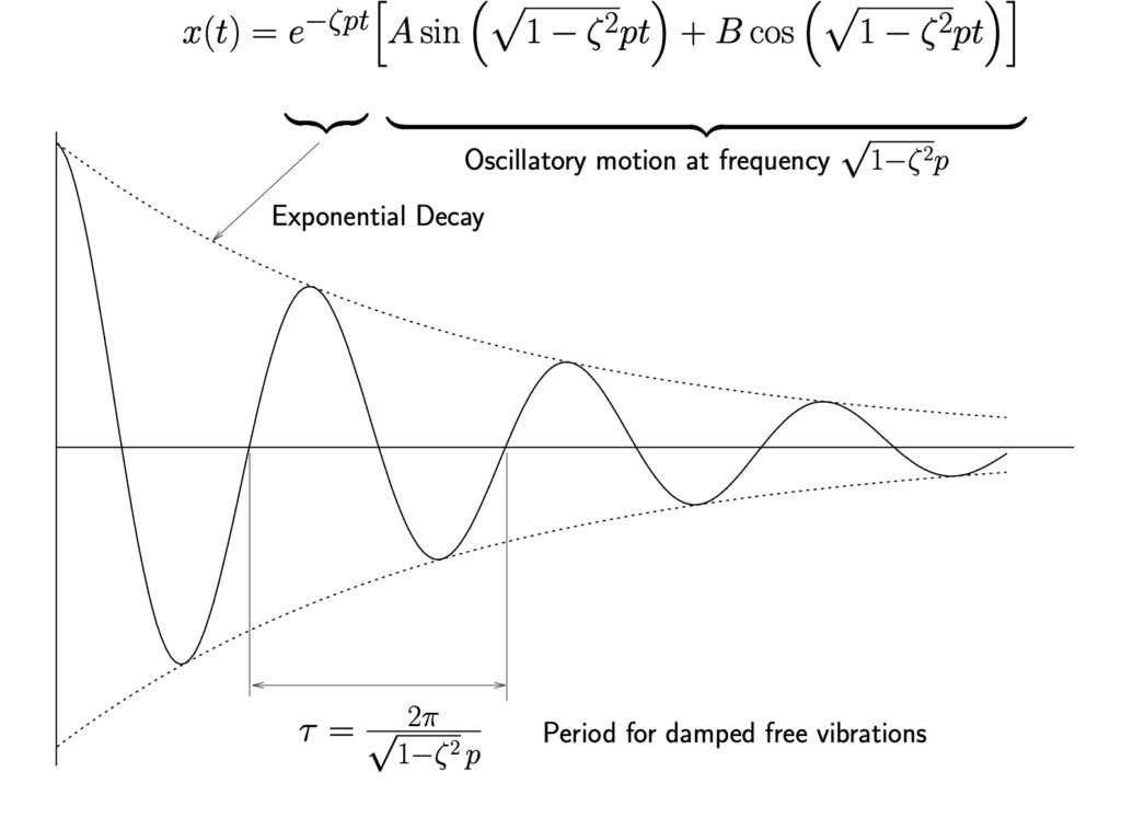
(3.11) $\begin{align*}x(t) &= e^{-\zeta p t} \Bigl[A \sin \left(\sqrt{1-\zeta^2}p t\right) + B \cos \left(\sqrt{1-\zeta^2}p t\right)\Bigr] \\\end{align*}$

or equivalently as

(3.12) $\begin{align*}x(t) &= e^{-\zeta p t} \Bigl[\mathbb{X} \sin \left(\sqrt{1-\zeta^2} p t + \phi \right) \Bigr]\end{align*}$

The $e^{-\zeta p t}$ term indicates that the amplitude of the response will decay with time, which agrees with our everyday experience with damped systems. A typical response is shown in Figure 3.2.

If the system has initial conditions given by

$\begin{equation*}x(0) = x_0, \qquad \dot{x}(0) = v_0,\end{equation*}$

it can be shown that the constants in equation 3.11 become

$\begin{equation*}A = \frac{v_0 + \zeta p x_0}{\sqrt{1-\zeta^2} p}, \qquad B = x_0,\end{equation*}$

so the complete response (for $t > 0$ ) can be written

(3.13) $\begin{equation*}x(t) = e^{-\zeta p t} \Biggl[\frac{v_0 + \zeta p x_0}{\sqrt{1-\zeta^2} p} \sin \left(\sqrt{1-\zeta^2} p t\right) +x_0 \cos \left(\sqrt{1-\zeta^2} p t\right)\Biggr]\end{equation*}$

The following tool demonstrations the free vibration response of a damped single degree of freedom system. Adjust the Displacement and/or Velocity terms to set the initial conditions. Adjust the mass, damping ratio, and stiffness to see the effect on the response. Use the play button to see the animation of the response.

EXAMPLE

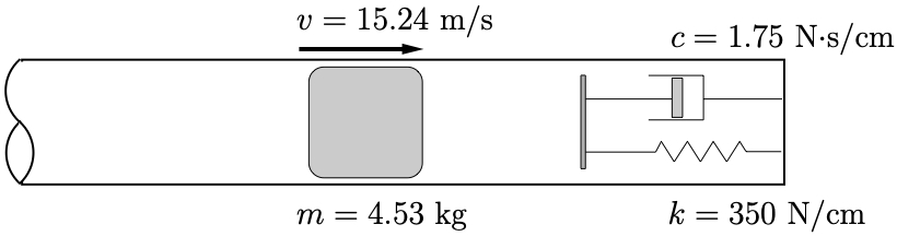
A piston with mass 4.53 kg is traveling in a smooth tube with a velocity of 15.24 m/s and engages a spring and damper as shown.

Determine how long it takes the piston to reach its maximum displacement after it engages the spring–damper.
Determine the maximum displacement.

Logarithmic Decrement

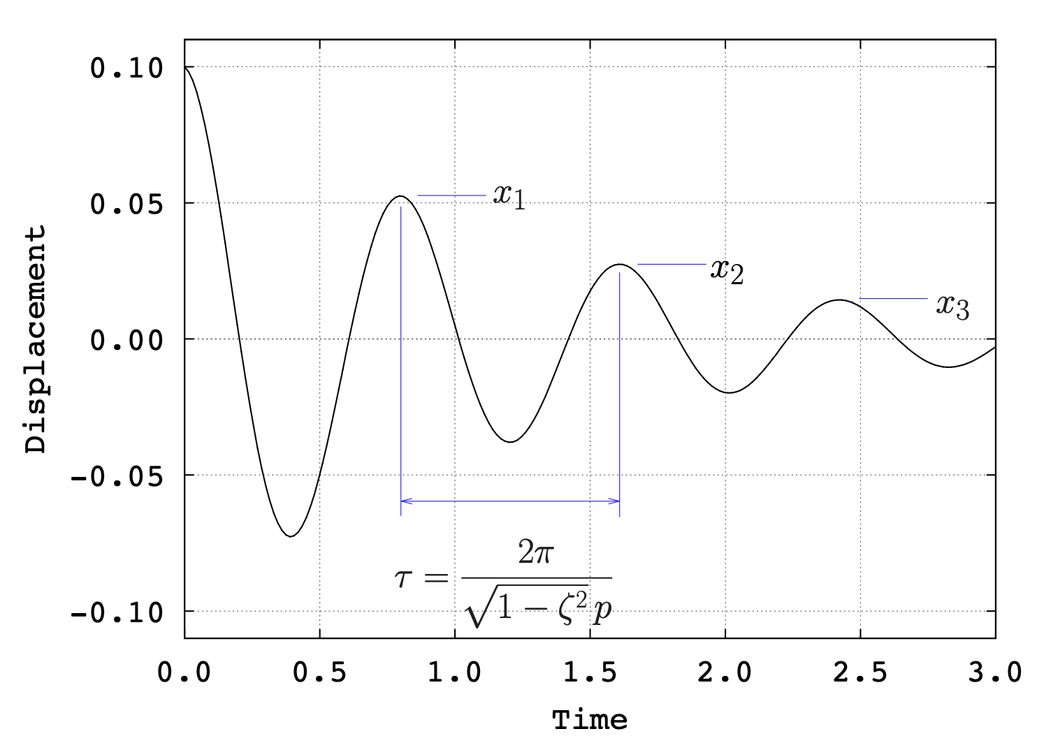
Figure 3.3: Ratios of successive peaks in an underdamped response

For an underdamped system, we can determine the damping ratio by considering the ratio of any two successive peaks in the response, such as $\frac{x_1}{x_2}$ shown in Figure 3.3. (The ratio $\frac{x_2}{x_3}$ could be used equally as well.) Using 3.12 this ratio can be written

(3.14) $\frac{x_1}{x_2} =\frac{e^{-\zeta p t_1} \left[ \cancel{\mathbb{X}} \sin \left(\sqrt{1-\zeta^2}p t_1 + \phi \right) \right]}{e^{-\zeta p t_2} \left[ \cancel{\mathbb{X}} \sin \left(\sqrt{1-\zeta^2}p t_2 + \phi \right) \right]}$

where $t_1$ and $t_2$ are times at which the peaks $x_1$ and $x_2$ occur respectively. Since these are peaks, these will occurs in the same part of the cycle (i.e. the times $t_1$ and $t_2$ are separated by one period exactly) so that $t_2 = t_1 + \tau$ where $\tau$ is the period for damped oscillations given by

(3.15) $\begin{equation*}\tau = \frac{2 \pi}{\sqrt{1-\zeta^2}\p}\end{equation*}$

As a result, the $\sin$ terms in 3.14 cancel and equation 3.14 further simplifies to

$\frac{x_1}{x_2} =\frac{e^{-\zeta p t_1}}{e^{-\zeta p t_2}}=\frac{e^{-\zeta p t_1}}{e^{-\zeta p (t_1 + \tau)}}=\frac{\cancel{e^{-\zeta p t_1}}}{\cancel{e^{-\zeta p t_1}} \cdot e^{-\zeta p \tau}}=\frac{1}{e^{-\zeta p \tau}} \\$

$\begin{equation*}\frac{x_1}{x_2} = e^{\zeta p \tau}\end{equation*}$

Taking the natural logarithm of both sides of this equations yields

(3.16) $\begin{equation*}\ln \frac{x_1}{x_2} = \zeta p \tau\end{equation*}$

Defining

(3.17) $\begin{equation*}\boxed{\delta \equiv \ln \frac{x_1}{x_2}}\end{equation*}$

and using the expression for the damped period in equation 3.15, 3.16 becomes

$\begin{equation*}\delta = \zeta p \biggl(\frac{2 \pi}{\sqrt{1-\zeta^2} p}\biggr)\end{equation*}$

(3.18) $\begin{equation*}\boxed{\delta = \frac{2 \pi \zeta}{\sqrt{1-\zeta^2}}}\end{equation*}$

which can be solved for $\zeta$ as

(3.19) $\begin{equation*}\boxed{\zeta = \frac{\delta}{\sqrt{\left( 2 \pi \right)^2 + \delta^2}}}\end{equation*}$

Note that for small damping values ( $\zeta \ll 1$ ), a good approximation is

$\begin{equation*}\zeta \approx \frac{\delta}{2 \pi}\end{equation*}$

Finally, note that we can also apply this approach using peaks which are $m$ cycles apart (peaks $x_n$ and $x_{n+m}$ ). (The peaks $x_1$ and $x_3$ in Figure 3.3 are two cycles apart for example). In this case the time between peaks is given by

$\begin{equation*}t_{n+m} - t_{n} = m \tau\end{equation*}$

and following a similar development to that above we can show that

$\begin{equation*}\frac{x_{n}}{x_{n+m}} = e^{m \zeta p \tau}\end{equation*}$

Taking the natural logarithm of both sides and again using equation 3.15 for the damped period results in

$\begin{equation*}\ln \frac{x_{n}}{x_{n+m}} = m \zeta p \biggl(\frac{2 \pi}{\sqrt{1-\zeta^2}\,p}\biggr)\end{equation*}$

$\begin{equation*}\frac{1}{m}\ln \frac{x_{n}}{x_{n+m}} = \frac{2 \pi \zeta}{\sqrt{1-\zeta^2}} \end{equation*}$

$\delta$ can now be defined more generally as

(3.20) $\begin{equation*}\boxed{\delta \equiv \frac{1}{m}\ln \frac{x_{n}}{x_{n+m}}}\end{equation*}$

so that

$\begin{equation*}\delta = \frac{2 \pi \zeta}{\sqrt{1-\zeta^2}}\end{equation*}$

which is identical to equation 3.18. As a result, equation 3.19 can again be used to determine the damping ratio $\zeta$ .

EXAMPLE

The following data are given for a vibrating system with viscous damping:

$\begin{equation*}w = 10~\mathrm{lb},\qquad & k = 30~\mathrm{lb/in},\qquad & c = 0.12~\mathrm{lb}\cdot\mathrm{s}/\mathrm{in}.\end{equation*}$

If the mass is given an initial displacement and then released, determine the logarithmic decrement and the ratio of any two successive amplitudes.

Critically Damped Response ( $\zeta = 1$ )

When $\zeta = 1$ , $\sqrt{\zeta^2-1} = 0$ so in this case the roots of the characteristics equation in 3.7 are repeated

$s_{1,2} = -\zeta \pm 0 = -\cancelto{1}{\zeta} = -1$

Since the roots are repeated, the solution to the governing equation requires the special form

(3.21) $\begin{equation*}x(t) = \Bigl( C_1 + C_2 t \Bigr) e^{-p t}\end{equation*}$

If the system has initial conditions given by

$\begin{equation*}x(0) = x_0, \qquad \dot{x}(0) = v_0\end{equation*}$

the constants $C_1$ and $C_2$ are

$\begin{equation*}C_1 = x_0, \qquad C_2 = v_0 + x_0 p\end{equation*}$

so the response becomes

(3.22) $\begin{equation*}x(t) = \Bigl[ x_0 + \bigl(v_0 + x_0 p \bigr) t \Bigr] e^{-p t}\end{equation*}$

Note that the response in equation 3.22 is not oscillatory, but due to the presence of the $e^{-p t}$ term the response will eventually decay to zero. For certain values of the initial conditions there may be one zero crossing, but the amplitude will decay to zero before another is made.

Overdamped Response ( $\zeta > 1$ )

When $\zeta > 1$ , the term $\sqrt{\zeta^2-1}$ will always be real, positive and smaller than $\zeta$ . As a result both of the roots in equation 3.7 will be real, negative and distinct and the response of the system is given by

(3.23) $\begin{equation*}x(t) = C_1 e^{\left(-\zeta + \sqrt{\zeta^2-1}\right) p t} +C_2 e^{\left(-\zeta - \sqrt{\zeta^2-1}\right) p t}\end{equation*}$

If the system has initial conditions given by

$\begin{equation*}x(0) = x_0, \qquad \dot{x}(0) = v_0,\end{equation*}$

then the constants $C_1$ and $C_2$ in equation 3.23 can be shown to be

$\begin{equation*}C_1 = \frac{ x_0 p \left( \zeta + \sqrt{\zeta^2-1} \right) + v_0}{2 p \sqrt{\zeta^2-1}},\qquad C_2 = \frac{-x_0 p \left( \zeta - \sqrt{\zeta^2-1} \right) - v_0}{2 p \sqrt{\zeta^2-1}}\end{equation*}$

so the response becomes

(3.24) $\begin{equation*}x(t) = \frac{ x_0 p\left( \zeta + \sqrt{\zeta^2-1} \right) + v_0}{2 p \sqrt{\zeta^2-1}}e^{\left(-\zeta + \sqrt{\zeta^2-1}\right) p t}+\frac{-x_0 p \left( \zeta - \sqrt{\zeta^2-1} \right) - v_0}{2 p \sqrt{\zeta^2-1}}e^{\left(-\zeta - \sqrt{\zeta^2-1}\right)p t}\end{equation*}$

Note that in this case the motion is once again non-oscillatory and that the motion will eventually decay and the system will approach the equilibrium position. This will take longer than in the critically damped case which reaches the equilibrium position in the shortest amount of time for any given set of initial conditions.

Open Educational Resources