
Sound and Acoustics: Sound Pressure Measurements
When sound pressure measurements are made, most commonly the actual pressure amplitudes are not measured directly. Instead, an effective pressure known as the root mean square pressure is used.
Root Mean Square Pressure Values
The root mean square pressure ( ) is defined as
(12.16) 
This is equivalent to the square root of the average of the pressure squared
![\begin{equation*} \ensuremath{P_{\text{RMS}}} = \sqrt{\bigl[ P^2 \bigr]_\text{AVE}} \end{equation*}](https://engcourses-uofa.ca/wp-content/ql-cache/quicklatex.com-fae095c462b58141d6d3d160080fe2e1_l3.png "Rendered by QuickLaTeX.com")
which is not the same as the square root of the square of the average pressure
![\begin{equation*} \ensuremath{P_{\text{RMS}}} \neq \sqrt{\bigl[ P_\text{AVE} \bigr]^2} . \end{equation*}](https://engcourses-uofa.ca/wp-content/ql-cache/quicklatex.com-a7134ad0f2c551206b1afe5548c36e5d_l3.png "Rendered by QuickLaTeX.com")
For a harmonic pressure wave given by

we have

so that

where  is the associated period given by

Therefore

(12.17) 
These relationships are illustrated in Figure 12.2.
Note that if we have a sound composed of several harmonic waves

where

then it can be shown that the RMS pressure of the resultant wave is given by

where

Note that this only applies if the sound sources are uncorrelated.
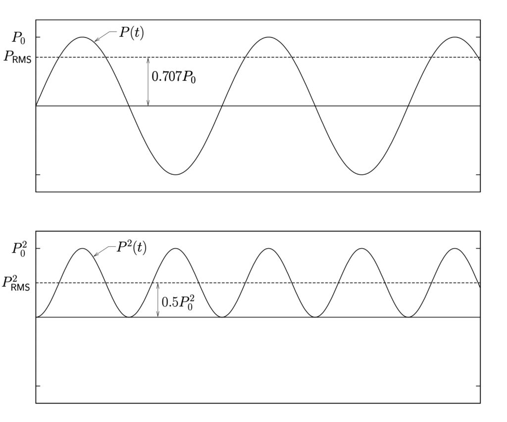
Figure 12.2: Root Means Square (RMS) pressure for harmonic waves
Superposition of Sound Waves
When two sound waves are superimposed, the result is a linear combination of the two individual waves due to the linearity of the wave equation. Two interesting situations which may occur, depending on the frequencies and amplitude of the two waves are
- Beating,
- Standing waves.
Beating
Beating occurs when two sounds of nearly the same frequency are combined. Consider two pressure waves with identical amplitudes and slightly different frequencies

When these two pressure waves are added together the total pressure is

or, using trigonometric identities,

(12.18) 
this pressure response becomes
(12.19) 
where

is the average of the two frequencies. If the difference between the two frequencies is small,  will be small (much smaller than
  ) so that the response can be interpreted as a wave whose frequency is the average of the two close frequencies, but which has a slowly varying amplitude. The beating period
  is defined as

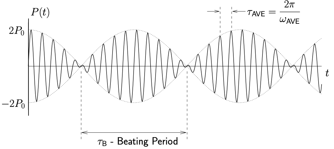
Figure 12.3: Beating response for two superimposed pressure waves
A typical beating response is shown in Figure 12.3. This is similar to the beating phenomenon discussed earlier.
Standing Waves
Standing waves can occur when two waves travel in opposite directions. This can occur when a sound wave reflects off a surface perpendicular to the direction of the original wave propagation.
Consider two waves of equal frequency and amplitude traveling in opposite directions (These can both be shown to satisfy the wave equation 12.5.)
![\begin{align*} P_1(t) &= P_0 \sin{\frac{\omega}{\ensuremath{c}} \bigl( x + \ensuremath{c} t \bigr)}, \\[2mm] P_2(t) &= P_0 \sin{\frac{\omega}{\ensuremath{c}} \bigl( x - \ensuremath{c} t \bigr)}. \end{align*}](https://engcourses-uofa.ca/wp-content/ql-cache/quicklatex.com-05f72573b4a1ccea1ca6182a25a21703_l3.png "Rendered by QuickLaTeX.com")
The superposition of these two waves results in
![\begin{align*} P(t) &= P_1(t) + P_2(t), \\ &= P_0 \sin{\frac{\omega}{\ensuremath{c}} \bigl( x + \ensuremath{c} t \bigr)} + P_0 \sin{\frac{\omega}{\ensuremath{c}} \bigl( x - \ensuremath{c} t \bigr)}, \\ &= P_0 \Bigl[ \sin{\frac{\omega x}{\ensuremath{c}}}\cos{\omega t} + {\cos{\frac{\omega x}{\ensuremath{c}}}\sin{\omega t}} + \sin{\frac{\omega x}{\ensuremath{c}}}\cos{\omega t} - {\cos{\frac{\omega x}{\ensuremath{c}}}\sin{\omega t}} \Bigr] \end{align*}](https://engcourses-uofa.ca/wp-content/ql-cache/quicklatex.com-390a99d0fabe5454ddd11a974fb4f481_l3.png "Rendered by QuickLaTeX.com")
(12.20) 
However, since  and
and  where
where  is the wavelength, we see that

so that 12.20 can be written
(12.21) ![\begin{equation*} P(t) = \underbrace{\Bigl[ 2 P_0 \sin{\frac{2 \pi x}{\lambda}} \Bigr]}_{\text{Amplitude}} %\underbrace{\cos{\omega t}}_{\text{Frequency of pressure wave}}. \cos{\omega t}. \end{equation*}](https://engcourses-uofa.ca/wp-content/ql-cache/quicklatex.com-768d85d723050a60b96012e9dd367e7c_l3.png "Rendered by QuickLaTeX.com")
Here we see that the amplitude of the pressure wave varies in space. In particular at locations given by

we see from 12.21 that  so there will be no sound at these locations.
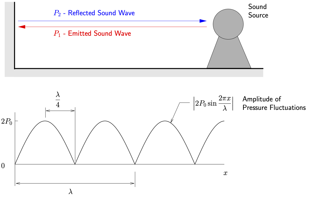
Figure 12.4: Illustration of standing waves.
Consider the situation shown in Figure 12.4. As can be seen, over the distance of  of the wavelength of the sound, the pressure amplitude can change from
  to 0. To put this in perspective, for sounds at 1000 Hz for example,
  \m so that
  cm. This can introduce large errors in the measurement of sound pressures. These kinds of errors can occur in industrial settings where reflective surfaces are present.