
Approximate Methods for Multiple Degree of Freedom Systems: Kinetic and Potential Energies in Multiple Degree of Freedom in Systems
So far we have considered multiple degree of freedom systems and have shown how to find the natural frequencies and modes shapes associated with such systems, which is essentially an eigenvalue problem. Often we are only interested in the lowest (or possibly the largest) natural frequency in a system. There are methods that can be used to estimate these frequencies which do not entail finding all of the natural frequencies of a system. We will discuss two such methods in this section, Rayleigh’s Quotient and Dunkerley’s Formula. To begin with, however, we need to consider how we can represent kinetic and potential energies in multiple degree of freedom systems.
Consider an  degree of freedom system with coordinates
  describing some displaced configuration of the system. Each
  may be a linear or angular displacement. Let

represent the values of the coordinates and their associated derivatives. For the linear systems considered here it can be shown that the potential energy in the system is given by
(9.1) ![\begin{equation*} U = \frac{1}{2} \bigl\{\!q\!\bigr\}\!\rule[4mm]{0pt}{0pt}^{T}\!\!\bigl[k\bigr]\! \bigl\{\!q\!\bigr\}\end{equation*}](https://engcourses-uofa.ca/wp-content/ql-cache/quicklatex.com-670af8981b1eb9ea9a4bbf31a5f235a6_l3.png "Rendered by QuickLaTeX.com")
where ![\bigl[k\bigr]](https://engcourses-uofa.ca/wp-content/ql-cache/quicklatex.com-2aab9db82919d8134feae5242052b74d_l3.png "Rendered by QuickLaTeX.com") is the stiffness matrix discussed earlier. Note that the potential energy is therefore zero at the equilibrium position. Similarly, the kinetic energy is given by
is the stiffness matrix discussed earlier. Note that the potential energy is therefore zero at the equilibrium position. Similarly, the kinetic energy is given by
(9.2) ![\begin{equation*}T = \frac{1}{2} \bigl\{\!\dot{q}\!\bigr\} ^{T} \!\!\bigl[m\bigr]\! \bigl\{\!\dot{q}\!\bigr\}\end{equation*}](https://engcourses-uofa.ca/wp-content/ql-cache/quicklatex.com-b416388f4a4b839a3e7ed99275cfc51f_l3.png "Rendered by QuickLaTeX.com")
where ![\bigl[m\bigr]](https://engcourses-uofa.ca/wp-content/ql-cache/quicklatex.com-733313d5e0f56bcd4cc88051f9f20e88_l3.png "Rendered by QuickLaTeX.com") is the mass matrix.
is the mass matrix.
EXAMPLE
At some instant in time, the masses in the system shown below are in positions  and
and  and have velocities
  and
and  , respectively.
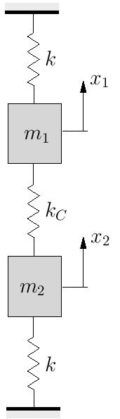
a) Determine the potential and kinetic energies in the system in terms of , , , and from first principles.
b) Show that the potential and kinetic energies can also be expressed as
![\[\begin{split}U &= \frac{1}{2}\left\{q\right\}^T\left[k\right]\left\{q\right\} \\T &= \frac{1}{2}\left\{\dot{q}\right\}^T\left[m\right]\left\{\dot{q}\right\}\end{split}\]](https://engcourses-uofa.ca/wp-content/ql-cache/quicklatex.com-9658c791b5c93ea09a1a62f0837837c6_l3.png "Rendered by QuickLaTeX.com")
where
![\[\begin{split}\left[k\right] &= \begin{bmatrix} k+ k_C & -k_C\\ -k_C & k+k_C \end{bmatrix}\\\left[m\right] &= \begin{bmatrix} m_1 & 0\\ 0 & m_2 \end{bmatrix}\end{split}\]](https://engcourses-uofa.ca/wp-content/ql-cache/quicklatex.com-8b988b0c0e7fee1a32c7216e4973c4ec_l3.png "Rendered by QuickLaTeX.com")
and
![\[\left\{q\right\} = \begin{Bmatrix} x_1 \\ x_2 \end{Bmatrix}, \qquad\left\{\dot{q}\right\} = \begin{Bmatrix} \dot{x}_1 \\ \dot{x}_2 \end{Bmatrix}\]](https://engcourses-uofa.ca/wp-content/ql-cache/quicklatex.com-b9d4f85963db380280938971cc80132a_l3.png "Rendered by QuickLaTeX.com")