Engineering at Alberta Courses » Simple Spring-Mass System

Forced Vibrations of Undamped Single Degree of Freedom Systems: Simple Spring-Mass System

The vibrations we have considered so far have all been free vibrations in which the system oscillates on its own without the presence of any external forces. One of the most important features of such systems is that they possess a natural frequency at which these free vibrations occur.

In many engineering applications the vibrations are caused by the action of an external force. The external force supplies energy to the system and drives the vibrations. These situations are term forced vibrations. The forcing function can take many forms, including

harmonic forces (periodic),
other periodic forces,
non-periodic forces.

We will begin our discussion by considering undamped systems acted upon by harmonic forces of the form

$\begin{equation*}F(t) = F_0 \sin{\omega t}\end{equation*}$

where

$F_0 =$ magnitude of the forcing function (N),
$\omega$ = frequency of the forcing function (rad/s).

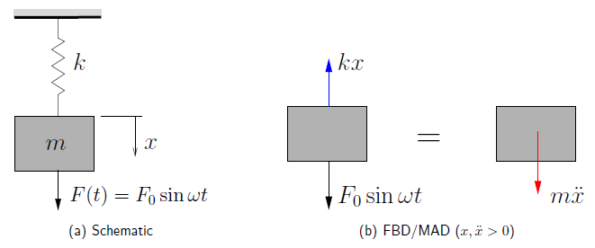
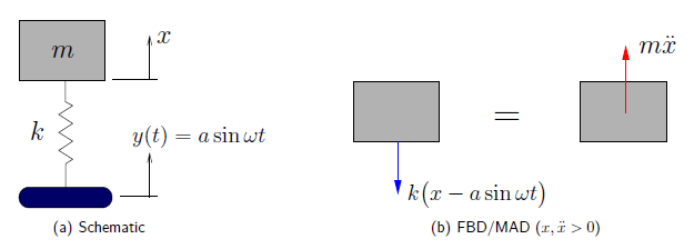
Consider a simple spring–mass system subjected to a harmonic force as shown in Figure 4.1(a). A FBD/MAD for this system is shown in Figure 4.1(b). (Note here that $x$ is the displacement from the static equilibrium position so we ignore the effect of gravity and the static stretch in the spring.) Applying Newton’s Laws the equation of motion for this system is

$\begin{equation*}+\!\!\downarrow\sum F = ma:\qquad F_0 \sin{\omega t} - kx = m \ddot{x}\end{equation*}$

(4.1) $\begin{equation*}m \ddot{x} + kx = F_0 \sin{\omega t}\end{equation*}$

This is the governing differential equation of motion for this system. It is similar to the equation of motion for free vibrations considered earlier, but the right–hand side is not zero (i.e. the equation is not homogeneous). As a result, we know that the solution to equation 4.1 is made up of two parts

(4.2) $\begin{equation*}x(t) = \underbrace{x_H(t)}_{{\substack{\text{Homogeneous}\\\text{Solution}}}} + \underbrace{x_P(t)}_{{\substack{\text{Particular}\\\text{Solution}}}}\end{equation*}$

where $x_H(t)$ is the homogeneous solution to the equation

$\begin{equation*}m \ddot{x}_H + k x_H = 0\end{equation*}$

We have already solved this problem and shown that the general solution is

(4.3) $\begin{equation*}x_H(t) = A \sin{pt} + B \cos{pt}\end{equation*}$

where as before $p$ is the natural frequency given by

$\begin{equation*}p = \sqrt{\frac{k}{m}}\end{equation*}$

and $A$ and $B$ are arbitrary constants. (Note that the natural frequency of a system does not change if a load is applied). $x_P(t)$ is known as the particular solution to 4.1 and depends on the exact form of the RHS. To find the particular solution in this case, we assume a solution which has the same `form’ as the RHS,

$\begin{equation*}x_P(t) = C \sin{\omega t}\end{equation*}$

so that

$\begin{equation*}\ddot{x}_P(t) = - C \omega^2 \sin{\omega t}\end{equation*}$

Substituting these into 4.1 results in

$m \Bigl[ - C \omega^2 \cancel{\sin{\omega t}} \Bigr] + k \Bigl[ C \cancel{\sin{\omega t}} \Bigr] &= F_0 \cancel{\sin{\omega t}} \\$

$C \Bigl(k - m \omega^2\Bigr) &= F_0$

so that

$\begin{equation*}C = \frac{F_0}{k-m\omega^2}\end{equation*}$

Therefore the particular solution is

(4.4) $\begin{equation*} x_P(t) = \frac{F_0}{k-m\omega^2} \sin{\omega t}\end{equation*}$

Substituting 4.3 and 4.4 into equation 4.2 gives the total solution for the response of the system as

(4.5) $\begin{equation*}x(t) = A \sin{p t} + B \cos{pt} + \frac{F_0}{k-m\omega^2} \sin{\omega t}\end{equation*}$

Note the following characteristics of the two parts of the solution.

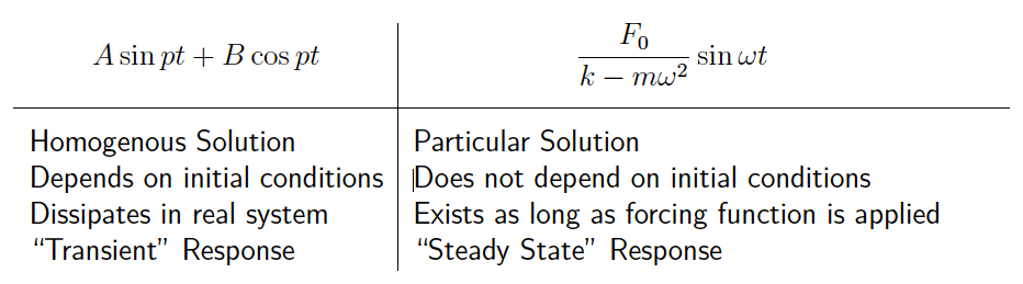
As discussed in the free vibration situation, the homogeneous response will eventually dissipate due to any damping in the system. Since all real systems have some damping, if we are only interested in the long term steady state response of the system we are often motivated to simply ignore the transient part of the solution and consider only the steady state response. This will not be a valid assumption early in the motion (i.e. shortly after the forcing function has been applied), but after a certain amount of time it will come to represent the true motion more appropriately.

Note that there is a bit of an inconsistency here in that we are neglecting the transient response because of damping in the system, but we started out by ignoring the damping in our original model. Once again, our motivation for doing so it that all real systems have some damping so the transient solution will disappear, whatever our model predicts. For lightly damped systems, an undamped model is both reasonable and simpler to use. It will simply take longer for the transient response to damp out. We will discuss forced damped systems eventually.

For now we wish to focus on the long term response of the system, so we will consider the total solution to be simply the steady state part of the motion

$\begin{equation*}x(t) = x_P(t) = \frac{F_0}{k-m\omega^2} \sin{\omega t}\end{equation*}$

which is conveniently rewritten as

(4.6) $\begin{equation*}x(t) = \underbrace{\Bigl (\frac{F_0}{k}\Bigr) \biggl (\frac{1}{1- \bigl(\frac{\omega}{p}\bigr) ^2}) \biggr)}_{\text{Amplitude }\mathbb X} \sin{\omega t}\end{equation*}$

We see that the amplitude of the response can be considered as a product of two terms:

$\dfrac{F_0}{k} = \delta_{ST}$

This is the static defection that the system would undergo if a force with the magnitude of the forcing function were applied statically.

$\dfrac{1}{1- \bigl(\frac{\omega}{p}\bigr) ^2 }$

This term accounts for the dynamic nature of the application of the force. The absolute value of this term is called the Dynamic Magnification Factor (DMF). This term determines how much the amplitude of the static deflection is magnified due to the harmonic nature of the force being applied. Note that this term can be positive or negative.

In terms of just the magnitude, we can see that

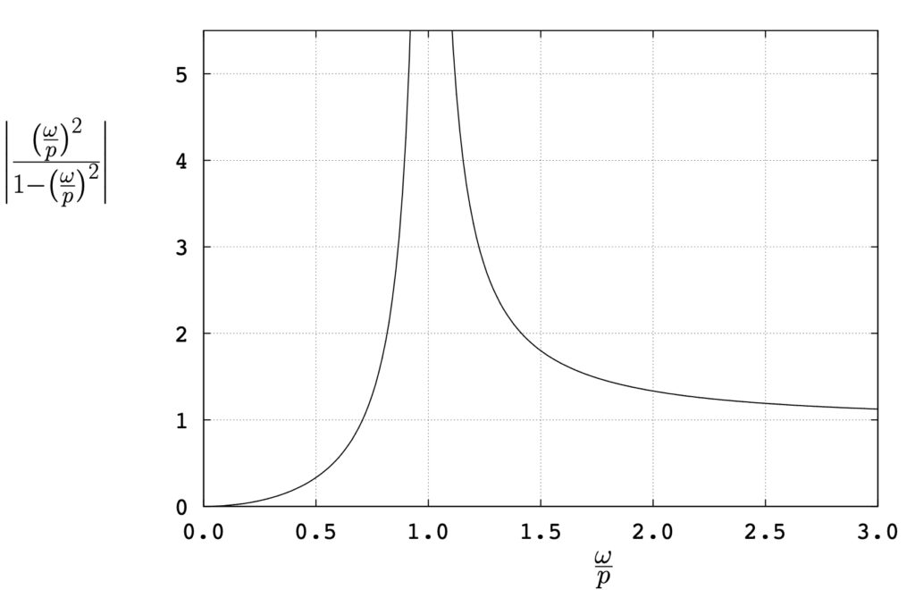
(4.7) $\begin{equation*}\mathbb X = \delta_{ST} \frac{1}{\left|1- \bigl(\frac{\omega}{p}\bigr) ^2\right|} \qquad\text{or}\qquad\boxed{\frac{\mathbb X}{\delta_{ST}} = \frac{1}{\left|1- \bigl(\frac{\omega}{p}\bigr) ^2\right|}}\end{equation*}$

These relations are shown in Figure 4.2(a) and (b).

(b) Dynamic Magnification Factor
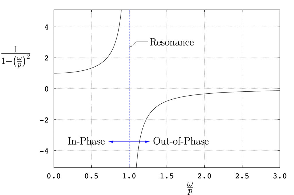
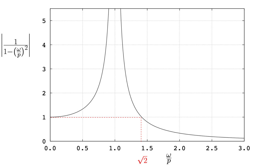
Figure 4.2: Steady state response of an undamped SDOF system

As can be seen in these figures, as $\omega\rightarrow 0$ , DMF $\rightarrow 1$ which is the static case. As $\frac{\omega}{p} \rightarrow 1$ , the amplitude of the response increases and approaches infinity. This situation, forcing a system at its natural frequency, is termed resonance and as can be seen leads to very large amplitudes of vibration. As $\frac{\omega}{p}$ gets large, the dynamic magnification factor approaches zero. For $\frac{\omega}{p} > \sqrt{2}$ , the amplitude of the response is less than the static deflection.

The tool below demonstrates the response for different values of $\frac{\omega}{p}$ . Use the slider to set the frequency ratio and press the play button to visualize the response.

If we now consider the sign of the response in equation 4.6, we see that it is positive when $\frac{\omega}{p}<1$ and negative when $\frac{\omega}{p}>1$ . This result means that for $\frac{\omega}{p}<1$ , $x$ is at a maximum value ( $\mathbb X$ ) when the forcing function is at a maximum value ( $\sin{\omega t} = 1$ ). Similarly, $x$ is at a minimum value ( $-\mathbb X$ ) when the forcing function is at a minimum ( $\sin{\omega t} = -1$ ).

In contrast, for $\omega p>1$ , the opposite situation occurs. $x$ is at a minimum value ( $-\mathbb X$ ) when the forcing function is at a maximum value ( $\sin{\omega t} = 1$ ) and is at a maximum value ( $\mathbb X$ ) when the forcing function is at a minimum ( $\sin{\omega t} = -1$ ). These situations are illustrated in Figure 4.3 below.

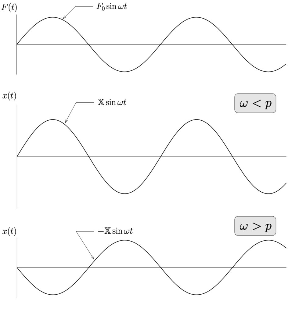
We say that when $\frac{\omega}{p} <1$ the forcing function and the response of the system are in–phase while for $\frac{\omega}{p} >1$ they are out–of–phase (by $\pi$ radians or completely out–of–phase). Another way to see this is to consider the response written in the form

$\begin{equation*}x(t) = \mathbb X \sin{(\omega t - \phi)}\end{equation*}$

where $\mathbb X$ is the magnitude of the response and $\phi$ represents the phase angle between the response and the forcing function (which is like $\sin\omega t$ in this case). For $\frac{\omega}{p}<1$ , the response is also like $\sin\omega t$ , so the forcing function and the response are in phase ( $\phi=0$ ) and the response can be written as

$\begin{equation*}x(t) =\mathbb X \sin{(\omega t - 0)}\end{equation*}$

For $\frac{\omega}{p}>1$ , the response is like $-\sin\omega t$ , and since

$\begin{equation*}-\sin\omega t = \sin{(\omega t - \pi)}\end{equation*}$

we could write the response

$x(t) = \Bigl(\frac{F_0}{k}\Bigr)\Biggl(\frac{1}{1- \bigl(\frac{\omega}{p}\bigr) ^2}\Biggr) \sin{\omega t}$

when $\frac{\omega}{p}>1$ as

$x(t) = -\Bigl(\frac{F_0}{k}\Bigr)\frac{1}{\Bigl|1- \bigl(\frac{\omega}{p}\bigr) ^2\Bigr|} \sin{\omega t}$

$= -\mathbb X \sin{\omega t}$

$x(t) = \mathbb X \sin{(\omega t - \pi)}$

where we can see that the phase angle is now $\pi$ radians (or 180°) which corresponds to a completely out-of-phase response. A plot of the phase angle $\phi$ as a function of the frequency ratio $\frac{\omega}{p} >1$ , is shown in Figure 4.4 below.

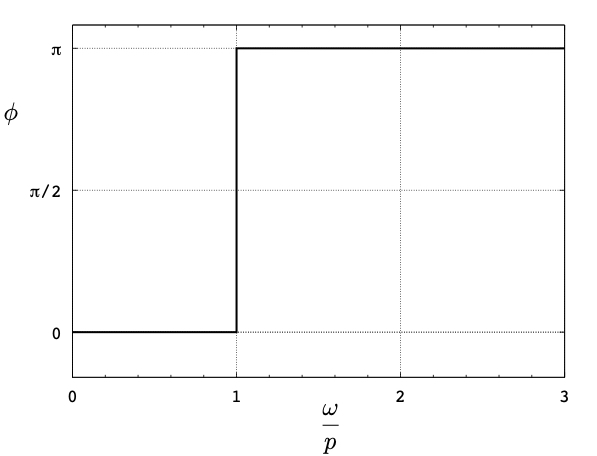
Figure 4.4: Phase angle in undamped situation

We will revisit this relationship when we consider the damped situation.

EXAMPLE

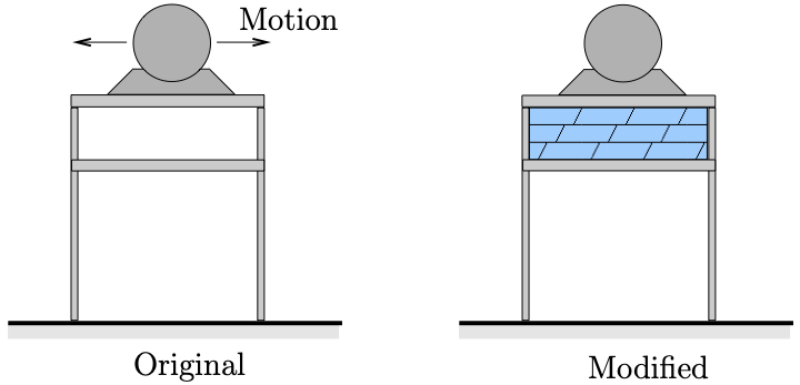
A steel frame supports a turbine-driven exhaust fan. At a speed of 400 RPM, the horizontal amplitude of the motion of the fan is 4.5 mm measured at the fan. At a speed of 500 RPM, the amplitude is 10 mm. No resonant condition is observed in changing the speed from 400 RPM to 500 RPM.

To decrease this excessive vibration, it is proposed to add a concrete slab under the fan to increase the mass of the system. Assuming the concrete slab doubles the effective mass,

Estimate the amplitude of the motion of the fan when operated at 400 RPM
Estimate the amplitude at 500 RPM.

Response at Resonance

The response of the system when it is forced at its natural frequency requires special treatment. If fact most of our results so far are not valid at the resonance condition $\omega=p$ . The problem is with the choice of particular solution. At resonance, the governing equation of motion becomes

$\begin{equation*}m \ddot{x} + kx = F_0 \sin{pt}\end{equation*}$

where we note that the forcing function is now at the natural frequency. The homogeneous solution to this equation does not change

$\begin{equation*}x_H(t) = A \sin{pt} + B \cos{pt}\end{equation*}$

so the total solution will be written

$\begin{equation*}x(t) = x_H(t) + x_P(t) = A \sin{pt} + B \cos{pt} + x_P(t)\end{equation*}$

At this point, however, we cannot choose a particular solution of the form

$\begin{equation*}x_P(t) = C \sin{pt}\end{equation*}$

as before because a $\sin{pt}$ term already exists as part of the homogeneous solution. This occurs only at resonance. In this case we instead assume a particular solution of the form

$\begin{equation*}x_P(t) = C t \sin{pt} + D t \cos{pt}\end{equation*}$

(note the extra $t$ in each term). Differentiating twice

$\begin{equation*}\ddot{x}_P(t) = 2 C p \cos{pt} - C t p^2 \sin{pt} - \Bigl[ 2 D p \sin{pt} + D t p^2 \cos{pt} \Bigr]\end{equation*}$

and substituting into the equation of motion gives

$\begin{equation*}m \Bigl[2 C p \cos{pt} - C t p^2 \sin{pt} - \Bigl( 2 D p \sin{pt} + D t p^2 \cos{pt}\Bigr)\Bigr] +k \Bigl[ C t \sin{pt} + D t \cos{pt} \Bigr] = F_0 \sin{pt}\end{equation*}$

Upon dividing by $m$ and noting that $\frac{k}{m} = p^2$ this simplifies to

(4.8) $\begin{equation*}2 C p \cos{pt} - 2 D p \sin{pt} = \frac{F_0}{m} \sin{pt}\end{equation*}$

Equating the $\sin{pt}$ and $\cos{pt}$ terms in 4.8 gives the result that

$\begin{equation*}C =0, \qquad D = -\frac{F_0}{2mp},\end{equation*}$

so that the complete response for the resonance condition is

$\begin{equation*}x(t) = A \sin{pt} + B \cos{pt} - \frac{F_0}{2mp} t \cos{pt}\end{equation*}$

where $A$ and $B$ can now be determined from initial conditions. To illustrate this response, if we assume for simplicity that the initial conditions are

$\begin{equation*}x(0) = 0, \qquad \dot{x}(0) = 0,\end{equation*}$

then the constants $A$ and $B$ become

$\begin{equation*}A = \frac{F_0}{2mp^2}, \qquad B=0,\end{equation*}$

and the total response becomes

(4.9) $\begin{equation*}x(t) = \frac{F_0}{2mp^2} \Bigl[ \sin{pt} - p t \cos{pt} \Bigr]\end{equation*}$

The presence of the $t$ in front of the $\cos{pt}$ term indicates that the response will continue to grow without bound as $t\rightarrow\infty$ . A plot of this response is shown in Figure 4.5.

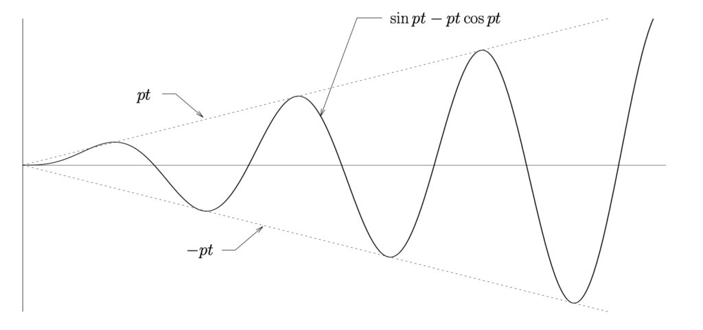
Our previous analysis indicated that the steady state response at the resonance condition is one with an infinite amplitude. As shown here however, we can see that the amplitude of the motion continually grows so that in reality a steady state solution of infinite amplitude is never reached. Any real structure would beak long before this occurred.

Forced Vibrations Due to a Rotating Imbalance

A common cause of forced vibrations in machinery is a rotating imbalance, which is shown schematically in Figure 4.6.

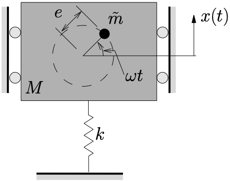
Figure 4.6: Schematic of a rotating imbalance

Here a machine with total mass $M$ is constrained to move in a vertical direction. $\tilde{m}$ is a rotating mass (which is included in the total mass $M$ ) with eccentricity $e$ that is rotating at a constant speed $\omega$ . During the resulting motion the machine body (the part that is not the eccentric mass) vibrates vertically, with a position described by the cooordinate $x(t)$ . The eccentric mass $\tilde{m}$ moves relative to the machine body. Its vertical component relative to the machine body is $e \sin{\omega t}$ as shown in Figure 4.6. The total vertical displacement of the eccentric mass is therefore $x + e \sin{\omega t}$ .

Figure 4.7 shows a FBD/MAD for this situation.

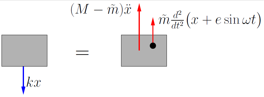
Applying Newton’s Laws in the vertical direction gives

$\begin{align*}+\!\!\uparrow\sum F = ma:\qquad-k x &= \bigl( M-\tilde{m} \bigr) \ddot{x} +\tilde{m} \dfrac{d^2}{d\,t^2} \bigl( x + e \sin{\omega t} \bigr) \\&= \bigl( M - {\tilde{m}} \bigr) \ddot{x} +\tilde{m} \bigl( {\ddot{x}} - e \omega^2\sin{\omega t} \bigr)\end{align*}$

(4.10) $\begin{equation*}M \ddot{x} + k x = \underbrace{\tilde{m}e\omega^2\rule[-1mm]{0pt}{0pt}}_{\textstyle F_0} \sin{\omega t}\end{equation*}$

This is the same equation of motion we obtained previously (equation 4.1) with

$\begin{equation*}F_0 = \tilde{m}e\omega^2\end{equation*}$

As a result we know the solution to the steady response is

$\begin{equation*}x(t) = \mathbb X \sin{(\omega t -\phi)}\end{equation*}$

where

(4.11) $\begin{equation*}\mathbb X = \frac{\dfrac{\tilde{m}e\omega^2}{k}}{\left|1- \bigl(\frac{\omega}{p}\bigr) ^2\right|}\end{equation*}$

and $\phi$ is either 0° or 180° depending on if the system is operating below or above resonance as discussed previously. Note however that since

$\frac{\tilde{m}e\omega^2}{k} = \frac{\tilde{m}e\omega^2}{k}\frac{M}{M} = \frac{\tilde{m} e}{M} \cancelto{\frac{1}{p^2}}{\frac{M}{k}} \omega^2,= \frac{\tilde{m} e}{M} \bigl(\frac{\omega}{p}\bigr) ^2$

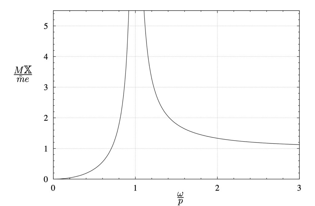
equation 4.11 can be rearranged to give

(4.12) $\begin{equation*}\boxed{\frac{M\mathbb X}{\tilde{m} e} = \frac{\bigl(\frac{\omega}{p}\bigr) ^2}{\bigl|1- \bigl(\frac{\omega}{p}\bigr) ^2\bigr|}}\end{equation*}$

This result, shown in Figure 4.8, is useful since it explicitly shows the parameters of interest, typically $M, \mathbb X$ and $\frac{\omega}{p}$ . There is no information here that is not available in 4.7 provided one uses $F_0 = \tilde{m}e\omega^2$ . The form shown here is can be easier to use in some situations.

This image has an empty alt attribute; its file name is undamped_rot_imbalance-1024x669.jpg — Figure 4.8: Response amplitude for a rotating imbalance

Note:

At slow speeds $\frac{\omega}{p}\rightarrow0$ , the disturbing force ( $\tilde{m}e\omega^2$ ) is small so the response is correspondingly small.
At very high speeds $\frac{\omega}{p}\gg1$ we can see that
$\begin{equation*}\frac{M\mathbb X}{\tilde{m} e} \approx 1 \qquad \text{so that} \qquad M\mathbb X \approx \tilde{m} e .\end{equation*}$

At these speeds the center of mass of the system remains approximately stationary. In a typical situation, $\tilde{m} << M$ so in essence the machine body remains approximately stationary. To see this, consider the specific instant when the eccentric mass is at its highest point relative to the machine body. Since $\frac{\omega}{p}>1$ , the response is out-of-phase and the machine body will be displaced downwards a distance $\mathbb X$ at this point, so the eccentric mass will have a net vertical displacement upwards of $(-\mathbb X + e)$ . The center of mass of the machine $\text{CM}$ , relative to the equilibrium position is given by

$\begin{align*}\text{CM} &= -\bigl( M-\tilde{m} \bigr) \mathbb X + \tilde{m} \bigl( -\mathbb X + e \bigr) \\&= -M\mathbb X + {\tilde{m}\mathbb X} - {\tilde{m} \mathbb X} + \tilde{m} e \\&= -M\mathbb X + \tilde{m} e \approx 0\end{align*}$

Base Excitation

So far we have considered the case in which a harmonic force is applied to the spring–mass system directly. A similar situation occurs when the \emph{base} supporting the spring undergoes harmonic motion, driven by some external force.

Consider such a situation shown in Figure 4.9(a). A FBD/MAD for this system is shown in Figure 4.9(b). ( $x$ is once again the displacement from the static equilibrium position so we ignore the effect of gravity and the static stretch in the spring.) Note that in an arbitrary configuration, the stretch in the spring (from the equilibrium position) is given by $x-a\sin{\omega t}$ . Applying Newton’s Laws we find

$\begin{equation*}+\!\!\uparrow\sum F = ma:\qquad -k\left(x-a\sin{\omega t}\right) = m \ddot{x}\end{equation*}$

(4.13) $\begin{equation*}m \ddot{x} + kx = k a \sin{\omega t}\end{equation*}$

This is the same equation of motion we obtained previously in the forced situation (equation 4.1) with

$\begin{equation*}F_0 = k a\end{equation*}$

As a result all of our previous results are applicable in this case as well. For example, the particular solution is

(4.14) $\begin{equation*}x(t) = a \biggl(\frac{1}{1- \bigl(\frac{\omega}{p}\bigr) ^2}\biggr) \sin{\omega t}\end{equation*}$

based on 4.6. In this case, the static deflection, previously shown to be $\delta_{ST} = \frac{F_0}{k}$ , becomes

$\delta_{ST} = \frac{F_0}{k} = \frac{{\cancel k} a}{{\cancel k}} = a$

which physically is the deflection the mass would undergo if the base were displaced quasi-statically. Similarly, the dynamic magnification factor we discussed previously now accounts for the effect of the base moving dynamically.

EXAMPLE

A vibrometer is a device used (unsurprisingly) to measure vibrations. A simple model of a vibrometer is shown below in which the device consists of a simple spring–mass system attached to the structure to be measured. A recording device within the vibrometer measures the relative motion $z$ between the structure and the vibrometer mass.

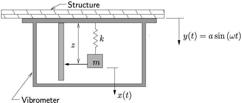
Determine the structure frequency $\omega$ above which the instrument can be used so that the measured amplitude $z$ will be within 2% of the structure’s true motion amplitude $a$

Transmissibility (Transmission Ratio, Force Transmissibility)

When a system undergoes vibration, significant forces can be generated. Transmissibility is a measure of how much force is transmitted to the supporting structure which is often a concern in vibrating systems. Transmissibility is defined as the ratio of the maximum force transmitted to the structure to the maximum disturbing force

$\begin{equation*}\boxed{TR = \frac{\text{Maximum force applied to supporting structure}}{\text{Maximum disturbing force}}.}\end{equation*}$

Harmonic Excitation

For a simple spring–mass system in Figure 4.1 acted upon by a harmonic force, the maximum disturbing force is $F_0$ (i.e. the magnitude of the harmonic force being applied). To determine the maximum force applied to the structure, we need to consider the response of the system since the only force applied to the structure is through the spring. Previously we found the steady state response to be

$\begin{equation*}x(t) = \mathbb X \sin{(\omega t -\phi)}\end{equation*}$

where

$\begin{equation*}\mathbb X = \frac{\dfrac{F_0}{k}}{\Bigl|1- \bigl(\frac{\omega}{p}\bigr) ^2\Bigl|}\end{equation*}$

The maximum force transmitted to the structure is then

$\begin{equation*}F_{Tmax} = k\mathbb X = \frac{F_0}{\Bigl|1- \bigl(\frac{\omega}{p}\bigr) ^2\Bigr|}\end{equation*}$

Therefore the transmissibility is

$\label{eq:TransSDOFUndamped}TR =\frac{F_{Tmax}}{F_{D}} = \frac{\dfrac{\cancel{F_0}}{\Bigl|1- \bigl(\frac{\omega}{p}\bigr) ^2\Bigr|}}{\cancel{F_0}} = \frac{1}{\Bigl|1- \bigl(\frac{\omega}{p}\bigr) ^2\Bigr|}$

In the case of the simple spring–mass system the transmissibility is the same as the dynamic magnification factor as shown in Figure 4.2(b).

Base Excitation

We can also consider transmissibility in the case of base excitation as illustrated in Figure 4.9. In this case we consider the maximum disturbing force to be

$\begin{equation*}F_D = k a\end{equation*}$

The force transmitted to the supporting structure can be seen to be

$\begin{equation*}F_T = k \bigl(x(t) - a \sin{\omega t} \bigr)\end{equation*}$

However, the steady state response of the mass in this situation has already been determined (equation 4.14) to be

$\begin{equation*}x(t) = \frac{a}{1- \bigl(\frac{\omega}{p}\bigr) ^2} \sin{\omega t}\end{equation*}$

As a result, the force transmitted to the support is therefore

$\begin{align*}F_T &= k \Biggl[\frac{a}{1- \bigl(\frac{\omega}{p}\bigr) ^2} \sin{\omega t} - a \sin{\omega t} \Biggr] \\&= k \Biggl[\frac{a}{1- \bigl(\frac{\omega}{p}\bigr) ^2} - a \Biggr] \sin{\omega t}\end{align*}$

The maximum force is therefore

$\begin{align*}F_T_{max} &= k \Biggl|\frac{a}{1- \bigl(\frac{\omega}{p}\bigr) ^2} - a \Biggr| \\&= k a \Biggl|\frac{1}{1- \bigl(\frac{\omega}{p}\bigr) ^2} - \frac{1- \bigl(\frac{\omega}{p}\bigr) ^2}{1- \bigl(\frac{\omega}{p}\bigr) ^2} \Biggr| \\&= ka \Biggl|\frac{{1 - 1} + \bigl(\frac{\omega}{p}\bigr) ^2}{1- \bigl(\frac{\omega}{p}\bigr) ^2} \Biggr| \\\end{align*}$

$\begin{equation*}F_T_{max} = ka \frac{\bigl(\frac{\omega}{p}\bigr) ^2}{\Bigl|1- \bigl(\frac{\omega}{p}\bigr) ^2\Bigr|}\end{equation*}$

and the transmissibility is then

$TR = \frac{F_T_{max}}{F_D} =\frac{\cancel{ka} \frac{\bigl(\frac{\omega}{p}\bigr) ^2}{\Bigl|1- \bigl(\frac{\omega}{p}\bigr) ^2\Bigr|}}{\cancel{ka}}$

(4.15) $\begin{equation*}\boxed{TR = \frac{\bigl(\frac{\omega}{p}\bigr) ^2}{\Bigl|1- \bigl(\frac{\omega}{p}\bigr) ^2\Bigr|}}\end{equation*}$

The transmissibility in this case is shown in Figure 4.10. Note that this is the same as shown in Figure 4.8 for the magnitude of the response in the rotating imbalance situation considered earlier.

This image has an empty alt attribute; its file name is base_excitation_transmissibility-1024x660.jpg — Figure 4.10: Transmissibility in undamped base excitation

EXAMPLE

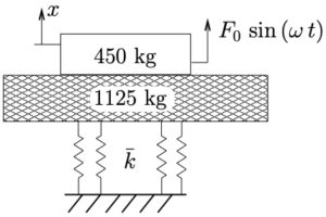
When an industrial machine with a mass of 450 kg was supported by springs (with negligible damping) it was found that the resulting static deflection was 5 mm. While the machine is running it is forced by a sinusoidally varying forcing function at a frequency of 1200 RPM.

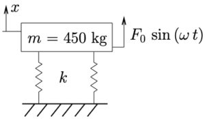
This image has an empty alt attribute; its file name is SDOF_Forced_Undamped_Ex_002_Fig_a-300x174.jpg

(a) What portion of the force acting on the machine is transmitted to the floor?

(b) If the machine is instead mounted on a 1125 kg concrete block, what portion of the force acting on the machine would be transmitted to the floor? What is the ratio of the amplitude of vibration now compared to before the concrete block was added?

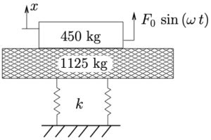
This image has an empty alt attribute; its file name is SDOF_Forced_Undamped_Ex_002_Fig_b-300x200.jpg

(c) If in addition to the concrete block stiffer springs $\bar{k}$ are used so that the static deflection is again 5 mm, what is the force transmissibility? What is the ratio of the amplitude of vibration compared to the original value?