
Transient Vibrations: Other Forcing Functions
So far we have considered the following forcing functions:
- harmonic,
- other periodic functions,
- step functions (including impulsive loading),
- ramp functions,
- exponential decay.
There are obviously many more we can come up with. Depending on the particular form of the forcing function, there are a number of ways of obtaining the response.
Simple Forcing Functions
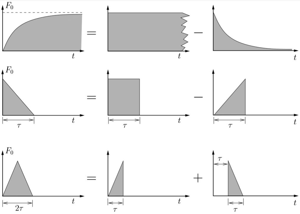
For other simple forcing functions, they can sometimes be represented as combinations of the types we have already seen.
In following this approach, we can sometime use superposition directly (as in the first two examples) or use two or more solutions sequentially where the final conditions for the first solution become the initial conditions for the second response.
Laplace Transforms
This approach transforms the differential equation into an algebraic equation which is significantly easier to solve in general. Once the solution is obtained, an inverse transform is performed to obtain the actual solution to the physical problem. This approach requires that the Laplace transform pairs are known for the particular forcing function of interest. We will not consider the use of Laplace transforms in this course, although they are very useful for vibration analysis and commonly used.
Convolution
This approach can be used for a general forcing function  and is based upon the response to impulsive loads that we have already discussed in equation (7.4). The method of convolution will be considered in the next section.
What impressed me most is the emphasis on choosing the appropriate mathematical technique based on the nature of the excitation rather than relying on a single solution method. Explaining composite forcing functions alongside Laplace transforms and convolution gives readers a much broader perspective on transient vibration analysis. It’s an outstanding resource for engineering students
Thank you for the comment!