
Multiple Degree of Freedom Systems: Semi-Definite Systems
In some systems the techniques shown so far do not work without modification. These occur when the system as a whole can move as a rigid body as well as vibrate. Such systems are known as semi-definite systems. They are also called degenerate or unrestrained systems.
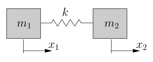
An example of such a system is shown in Figure 8.9. This could be a model of two train cars joined on a railway track for example.
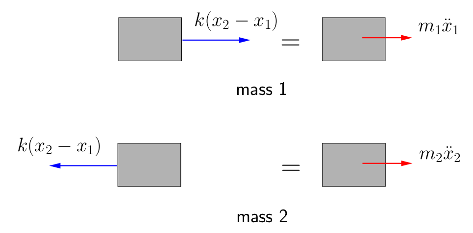
Figure 8.10 shows the FBD/MAD’s for the masses  and
and  . The equation of motion for mass 1 is
![\[\stackrel{+}{\rightarrow}\sum F = ma: \qquad k \bigl( x_2 - x_1 \bigr) = m_1 \ddot{x}_1\]](https://engcourses-uofa.ca/wp-content/ql-cache/quicklatex.com-97b0524054eea243e023db80c3bb926d_l3.png "Rendered by QuickLaTeX.com")
while for mass 2 we get
![\[\stackrel{+}{\rightarrow}\sum F = ma: \qquad -k \bigl( x_2 - x_1 \bigr) = m_2 \ddot{x}_2\]](https://engcourses-uofa.ca/wp-content/ql-cache/quicklatex.com-6c10744c6c3c135db564c02a75aa127f_l3.png "Rendered by QuickLaTeX.com")
In matrix form these become
(8.29) ![\[\begin{bmatrix}m_1 & 0 \\0 & m_2 \\\end{bmatrix}\!\!\biggl\{\!\!\!\begin{array}{c}\ddot{x}_1 \\ \ddot{x}_2 \\\end{array}\!\!\!\biggr\}+\biggl[\!\!\begin{array}{rr}k & -k \\-k & k \\\end{array}\!\!\biggr]\!\!\biggl\{\!\!\!\begin{array}{c}x_1 \\ x_2 \\\end{array}\!\!\!\biggr\}=\biggl\{\!\!\!\begin{array}{c}0 \\ 0 \\\end{array}\!\!\!\biggr\}\]](https://engcourses-uofa.ca/wp-content/ql-cache/quicklatex.com-009b09078d0c7309435aeedf39a5c97b_l3.png "Rendered by QuickLaTeX.com")
Assuming simple simultaneous harmonic motion of the form
![\[\biggl\{\!\!\!\begin{array}{c}x_1 \\ x_2 \\\end{array}\!\!\!\biggr\}=\biggl\{\!\!\!\begin{array}{c}\ensuremath{\mathbb{A}}_1 \\ \ensuremath{\mathbb{A}}_2 \\\end{array}\!\!\!\biggr\} \, \ensuremath{\sin\left(\ensuremath{p} t + \phi\right)}\]](https://engcourses-uofa.ca/wp-content/ql-cache/quicklatex.com-ce882e5d17f72fdb85cf5e84566dc9aa_l3.png "Rendered by QuickLaTeX.com")
we have
![\[\biggl\{\!\!\!\begin{array}{c}\ddot{x}_1 \\ \ddot{x}_2 \\\end{array}\!\!\!\biggr\}=- \ensuremath{p}^2 \biggl\{\!\!\!\begin{array}{c}\ensuremath{\mathbb{A}}_1 \\ \ensuremath{\mathbb{A}}_2 \\\end{array}\!\!\!\biggr\} \, \ensuremath{\sin\left(\ensuremath{p} t + \phi\right)}\]](https://engcourses-uofa.ca/wp-content/ql-cache/quicklatex.com-3ed959545924c2a81899acc25e27a607_l3.png "Rendered by QuickLaTeX.com")
so that (8.29) leads to
(8.30) ![\[\begin{bmatrix}k - m_1 \ensuremath{p}^2 & -k \\-k & k -m_2 \ensuremath{p}^2 \\\end{bmatrix}\!\!\biggl\{\!\!\!\begin{array}{c}\ensuremath{\mathbb{A}}_1 \\ \ensuremath{\mathbb{A}}_2 \\\end{array}\!\!\!\biggr\}=\biggl\{\!\!\!\begin{array}{c}0 \\ 0 \\\end{array}\!\!\!\biggr\}\]](https://engcourses-uofa.ca/wp-content/ql-cache/quicklatex.com-eefda68cb1e05aba7e9d6867ddb8372d_l3.png "Rendered by QuickLaTeX.com")
For a non-trivial solution we require the determinant to be zero, i.e.
![\begin{align*} \bigl(k - m_1 \ensuremath{p}^2\bigr)\bigl(k - m_2 \ensuremath{p}^2\bigr) - \bigl(-k\bigr)\bigl(-k\bigr) &= 0\\k^2 - k m_1 \ensuremath{p}^2 - k m_2 \ensuremath{p}^2 + m_1m_2\ensuremath{p}^4 - k^2 &= 0 \\\ensuremath{p}^2 \Bigl[ m_1m_2\ensuremath{p}^2 - k \bigl(m_1+m_2) \Bigr]&= 0\end{align*}](https://engcourses-uofa.ca/wp-content/ql-cache/quicklatex.com-47f25c5966417f2ea2b7c56bc3c1d069_l3.png "Rendered by QuickLaTeX.com")
which has the roots

The zero natural frequency corresponds to rigid body motion of the system. (Since the frequency is zero, the period is infinite indicating that vibrations do not occur – the system never returns to its starting point). To understand this further we can investigate the mode shapes associated with each of these frequencies. From the first equation in (8.30) we find
(8.31) ![\[\bigl(k - m_1 \ensuremath{p}^2\bigr)\ensuremath{\mathbb{A}}_1 - \bigl(k\bigr) \ensuremath{\mathbb{A}}_2 = 0\qquad\longrightarrow\qquad\frac{\ensuremath{\mathbb{A}}_2}{\ensuremath{\mathbb{A}}_1} = \frac{k - m_1 \ensuremath{p}^2}{k}\]](https://engcourses-uofa.ca/wp-content/ql-cache/quicklatex.com-b74b1972efddbfe5b464f78b99c5d170_l3.png "Rendered by QuickLaTeX.com")
For  ,
,
![\[\newcommand{\MODE}[1]{\ensuremath{\!\!\rule[5mm]{0pt}{0pt}^{\textcircled{{\footnotesize{#1}}}}}}\biggl(\!\frac{\ensuremath{\mathbb{A}}_2}{\ensuremath{\mathbb{A}}_1}\!\biggr)\MODE{1} = \frac{k - m_1 \ensuremath{p}^2}{k} = \frac{k}{k} = 1\qquad\longrightarrow\qquad\biggl\{\!\!\!\begin{array}{c}\ensuremath{\mathbb{A}}_1 \\ \ensuremath{\mathbb{A}}_2 \\\end{array}\!\!\!\biggr\}\MODE{1}=\biggl\{\!\!\!\begin{array}{c}1 \\ 1 \\\end{array}\!\!\!\biggr\}\]](https://engcourses-uofa.ca/wp-content/ql-cache/quicklatex.com-bd38525fe54d401d037e3adb7544cd85_l3.png "Rendered by QuickLaTeX.com")
For  ,
,
![\[\newcommand{\MODE}[1]{\ensuremath{\!\!\rule[5mm]{0pt}{0pt}^{\textcircled{{\footnotesize{#1}}}}}}\biggr(\frac{\mathbb{A}_2}{\mathbb{A}_1}\biggl)\MODE{2}=\frac{k-m_1p^2}{k}=\frac{-m_1}{m_2}\,\rightarrow\,\biggr\{\frac{\mathbb{A}_2}{\mathbb{A}_1}\biggl\}\MODE{2}=\biggr\{\frac{1}{\frac{-m_1}{m_2}}\biggl\}\]](https://engcourses-uofa.ca/wp-content/ql-cache/quicklatex.com-078db9a6c9a2facbbdd635088469e1d6_l3.png "Rendered by QuickLaTeX.com")
The first mode shape corresponds to rigid body motion of the system. Since both cars are always displaced the same distance in the same direction, there will be no distortion of the spring. With no stretch in the spring, the equations of motion simplify to
![\[\begin{Bmatrix} \ddot{x}_1 \\ \ddot{x}_2 \end{Bmatrix} = \begin{Bmatrix} 0 \\ 0 \end{Bmatrix}\]](https://engcourses-uofa.ca/wp-content/ql-cache/quicklatex.com-e3c594b0ab767639fed35d6d18aab8e7_l3.png "Rendered by QuickLaTeX.com")
which have the general solutions

where  and
and  are obtained from the initial conditions. The initial conditions corresponding to this mode are
 – spring is initially unstretched
 – each car has the same initial velocity.
If the system is started with these conditions, then the cars will simply move as a rigid body at constant velocity (i.e. no vibrations will occur as the spring has no effect at all).
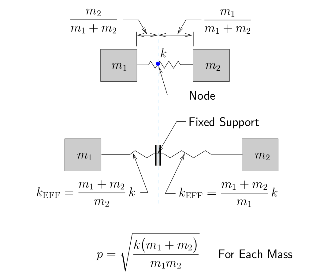
For the second mode shape we see that the masses will move in opposite directions with the relative amplitudes depending on the ratio of the two masses. If  , mass 1 will have a greater amplitude of motion than mass 2 and vice versa. In this mode there will be a point on the spring that does not move. This point, referred to as a node will be located a fraction
  the distance along the spring from mass 1 as shown in Figure 8.11. If , this point will be closer to mass 1. As we have seen previously, for a system vibrating in this mode, this point which does not move is equivalent to a fixed support so we could interpret this as two independent single degree of freedom systems, each with a frequency of
  as illustrated in Figure 8.11.
Note that for semi-definite systems:
- We cannot treat these semi-definite systems using normal matrix methods since the stiffness matrix itself is singular. This is always the case for these systems.
- A semi-definite system can have more than one rigid body mode, but the most it can have is six, corresponding to three translations in space and three rotations about perpendicular axes.
- There are techniques that can be used to remove the rigid body modes from the system so that standard analysis techniques can be used. These are beyond the scope of this course however.