
Sound and Acoustics: Sound Propagation
Sound Propagation in One Dimension
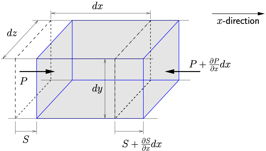
Figure 12.1: Compression wave travelling in  -direction
We begin by considering a longitudinal compression wave traveling in a fluid in the -direction. An infinitesimal element with initial dimensions  and
and  is shown in Figure 12.1. This fluid element will deform as the wave passes and a deformed configuration of the fluid element is shown highlighted in gray. Here
  represents the displacement of the fluid in the -direction while
  is the acoustic overpressure in the fluid (i.e. the pressure above the local atmospheric (equilibrium) pressure). At the left end of the deformed fluid element in Figure 12.1 the material has displaced an amount
  and is acted upon by a pressure
  . At the right end, the displacement and pressure are

and

respectively.
Application of Newton’s law in the -direction results in
![\begin{align*} \stackrel{+}\rightarrow\sum F = ma: \qquad {P \,dy\,dz} - \biggl({P} + \frac{\partial P}{\partial x} dx\biggr) dy\,dz &= \underbrace{\rho \, dx \, dy \, dz\rule[-2mm]{0pt}{0pt}}_{\normalsize dm} \, \frac{\partial^2 S}{\partial t^2}, \\ -\frac{\partial P}{\partial x} \,{dx\,dy\,dz} &= \rho \, {dx \, dy \, dx} \, \frac{\partial^2 S}{\partial t^2}, \nonumber \end{align*}](https://engcourses-uofa.ca/wp-content/ql-cache/quicklatex.com-68f192da96409dbfd5e404aedbf53224_l3.png "Rendered by QuickLaTeX.com")
(12.1) 
We assume that the pressure (above atmospheric) is related to the volumetric strain by
(12.2) 
where  is the bulk modulus of the fluid. Since the only motion of the fluid element is in the -direction, we see that

so that 12.2 becomes
(12.3) 
and 12.1 becomes

or
(12.4) 
This is the wave equation which governs the displacement of the fluid. To consider the response of the pressure, we begin by differentiating 12.1 with respect to

Using the result from 12.3 this becomes

which can be rearranged to give
(12.5) 
Comparing 12.4 and 12.5 we see that both the displacement and the pressure satisfy the same wave equation. The wave speed in both cases is given by
(12.6) 
This speed is known as the speed of sound in the medium.
Speed of Sound
Generally in acoustics we are concerned with the transmission of sound through air. Under most conditions of interest, air can be treated as an ideal gas so that
(12.7) 
Here  is the total pressure of the air given by
(12.8) 
where  is the atmospheric pressure and is the acoustic overpressure.
  in 12.7 is the absolute temperature and
  is the ideal gas constant which for air is

Bulk Modulus
As we saw in 12.2, the change in pressure of a gas is related to the volumetric strain according to

(12.9) 
Pressure fluctuations of this sort are an adiabatic (no heat transfer) process which for an ideal gas follow
(12.10) 
where  is the ratio of specific heats (
  ). Differentiating 12.10 with respect to volume shows that

(12.11) 
Comparing 12.9 and 12.11 we see that for an ideal gas the bulk modulus is given by
(12.12) 
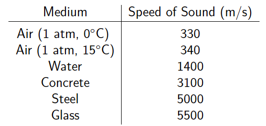
Table 12.1: Typical speed of sound in various media
From 12.6 we know that the speed of sound is related to the bulk modulus and density by

which using 12.12 becomes
(12.13) 
However, from the ideal gas law we know that

so that 12.13 becomes
![\[ \ensuremath{c} = \sqrt{\frac{\gamma \cancel{\tilde{P}}}{\biggl(\frac{\cancel{\tilde{P}}}{R\,T}\biggr)}} \]](https://engcourses-uofa.ca/wp-content/ql-cache/quicklatex.com-8391f80348aa6e77f68e9413aa8a01cd_l3.png "Rendered by QuickLaTeX.com")
(12.14) 
With  and
and  , this gives

in m/s where is the absolute temperature.
For a solid, the bulk modulus of a material is

where  is Young’s Modulus and
  is Poisson’s ratio. This represents how much a solid is compressed if acted upon by a hydrostatic stress state. Note that if
  , which is typical of many engineering materials, then the bulk modulus is approximately the same as Young’s Modulus. Table 12.1 shows the speed of sound in several media.
Frequency and Wavelength
The speed of sound is related to \itspos frequency and wavelength by
(12.15) 
where

Human hearing is nominally within the range of 20 Hz to 20 kHz. For air at 15 °C, ( = 340 m/s) this corresponds to wavelengths ranging from 17 m to 17 mm.


Out of interest we can compare this to human vision. The visible light spectrum ( = 3 m/s) nominally corresponds to


Notice that for the visible light spectrum the ratio of the maximum frequency to the minimum frequency is less than two. For human hearing this ratio is about 1000.