
Approximate Methods for Multiple Degree of Freedom Systems: Dunkerley’s Formula
Dunkerley’s Formula is another method of estimating the lowest (fundamental) natural frequency of a system without having to solve an eigenvalue problem. Rather than using the stiffness matrix, Dunkerley’s Method makes use of the flexibility matrix ![\bigl[a\bigr]](https://engcourses-uofa.ca/wp-content/ql-cache/quicklatex.com-5ff874b91b845fe10cca2937cf335e37_l3.png "Rendered by QuickLaTeX.com") which is the inverse of the stiffness matrix.
which is the inverse of the stiffness matrix.
Starting with the equations of motion for a general  degree of freedom system
![\begin{equation*}\bigl[m\bigr]\!\bigl\{\ddot{x}\bigr\} + \bigl[k\bigr]\!\bigl\{x\bigr\} = \bigl\{0\bigr\}\end{equation*}](https://engcourses-uofa.ca/wp-content/ql-cache/quicklatex.com-b7fe9bac35f8cbaf4038f0cab6535986_l3.png "Rendered by QuickLaTeX.com")
and assuming simple simultaneous harmonic motion of the form

results in
(9.9) ![\begin{equation*}-p^2 \bigl[m\bigr]\!\bigl\{\!\mathbb{A}\!\bigr\} + \bigl[k\bigr]\!\bigl\{\!\mathbb{A}\!\bigr\} = \bigl\{0\bigr\}\end{equation*}](https://engcourses-uofa.ca/wp-content/ql-cache/quicklatex.com-52f6f7b648a283729ffd18b6e9de219f_l3.png "Rendered by QuickLaTeX.com")
Premultiplication of (9.9) by ![\bigl[k\bigr]\!\!\rule[5mm]{0pt}{0pt}^{-1}](https://engcourses-uofa.ca/wp-content/ql-cache/quicklatex.com-707245e70fe89d6ad7c024e43ba38bd6_l3.png "Rendered by QuickLaTeX.com") results in
results in
![\begin{equation*}-\ensuremath{p}^2 \underbrace{\bigl[k\bigr]\!\!\rule[5mm]{0pt}{0pt}^{-1}}_{\bigl[a\bigr]}\bigl[m\bigr]\!\bigl\{\!\mathbb{A}\!\bigr\} + \underbrace{\bigl[k\bigr]\!\!\rule[5mm]{0pt}{0pt}^{-1}\bigl[k\bigr]}_{\bigl[1\bigr]}\!\bigl\{\!\mathbb{A}\!\bigr\} = \bigl\{0\bigr\}\end{equation*}](https://engcourses-uofa.ca/wp-content/ql-cache/quicklatex.com-f423d427f05adaa6bdde3ba9a01beb2c_l3.png "Rendered by QuickLaTeX.com")
so that
![\begin{equation*}\bigl[a\bigr]\!\bigl[m\bigr]\!\bigl\{\!\mathbb{A}\!\bigr\} - \frac{1}{\ensuremath{p}^2} \bigl\{\!\mathbb{A}\!\bigr\} = \bigl\{0\bigr\}\end{equation*}](https://engcourses-uofa.ca/wp-content/ql-cache/quicklatex.com-64b3b1fa74128c54ecf842b786388e81_l3.png "Rendered by QuickLaTeX.com")
or
![\begin{equation*}\biggl[\bigl[a\bigr]\!\bigl[m\bigr]- \frac{1}{\ensuremath{p}^2} \bigl[1\bigr] \biggr] \bigl\{\!\mathbb{A}\!\bigr\} = \bigl\{0\bigr\}\end{equation*}](https://engcourses-uofa.ca/wp-content/ql-cache/quicklatex.com-3cc733b8fbda62b8872e5fdd1f60968b_l3.png "Rendered by QuickLaTeX.com")
As we have seen previously, for a non-trivial solution to exist it is required that
(9.10) ![\begin{equation*}\biggl| \bigl[a\bigr]\!\bigl[m\bigr] - \frac{1}{p^2} \bigl[1\bigr] \biggr| = 0\end{equation*}](https://engcourses-uofa.ca/wp-content/ql-cache/quicklatex.com-a5c91f22fabfdc21e75534f201aec2c1_l3.png "Rendered by QuickLaTeX.com")
For simplicity we will assume that the mass matrix is diagonal. In that case, the determinant in (9.10) has the form
![\begin{equation*}\left| \left[\begin{matrix}a_{{1}{1}} & a_{{1}{2}} & \dots & a_{{1}{N}} \\a_{{2}{1}} & a_{{2}{2}} & \dots & a_{{2}{N}} \\\vdots & \vdots & \ddots & \vdots \\a_{{N}{1}} & a_{{N}{2}} & \dots & a_{{N}{N}} \\\end{matrix}\right]\left[\begin{matrix}m_1 & 0 & \dots & 0 \\0 & m_2 & \dots & 0 \\\vdots & \vdots & \ddots & \vdots \\0 & 0 & \dots & m_N \\\end{matrix}\right]-\left[\begin{matrix}\dfrac{1}{p^2} & 0 & \dots & 0 \\0 & \dfrac{1}{p^2} & \dots & 0 \\\vdots & \vdots & \ddots & \vdots \\0 & 0 & \dots & \dfrac{1}{p^2} \\\end{matrix}\right] \right|= 0\end{equation*}](https://engcourses-uofa.ca/wp-content/ql-cache/quicklatex.com-8b3c9e184e7b53caf902fdec93d6dbf1_l3.png "Rendered by QuickLaTeX.com")
or
(9.11) 
Expanding (9.11) produces the characteristic equation which has the form
(9.12) 
where  and
and  are constants (which will depend on and
 ![\bigl[m\bigr]](https://engcourses-uofa.ca/wp-content/ql-cache/quicklatex.com-733313d5e0f56bcd4cc88051f9f20e88_l3.png "Rendered by QuickLaTeX.com") ) which we do not need to consider here.
) which we do not need to consider here.
Let the roots of (9.12) be given by

Since these values are the roots, the characteristic equation could also be written in the form
(9.13) 
which is a completely equivalent polynomial to (9.12). Expanding (9.13) we get
(9.14) 
where and are the same constants which appeared in (9.12). Comparing the  terms in equations (9.12) and (9.14) shows that
(9.15) 
To this point no approximations have been made. Now however, we note that for many systems the higher natural frequencies are significantly larger than the fundamental natural frequency  so that

As a result, ignoring all but the first term on the LHS of (9.15) results in
![\[\frac{1}{p_1^2} + \cancelto{\mathrm{ignore}}{\frac{1}{p_2^2} + \dots +\frac{1}{p_N^2}} =a_{{1}{1}} m_1 + a_{{2}{2}} m_2 + \dots + a_{{N}{N}} m_N\]](https://engcourses-uofa.ca/wp-content/ql-cache/quicklatex.com-87c7c5c2a2ff73da8bb1b3256ec07cfd_l3.png "Rendered by QuickLaTeX.com")
or

or more generally
(9.16) 
Equation (9.16) is known as Dunkerley’s Formula and provides an estimate of the fundamental natural frequency of a system. Due to the terms that have been neglected, the natural frequency obtained using Equation (9.16) will be lower than the actual fundamental natural frequency. Dunkerley’s Formula therefore provides a lower bound on the lowest natural frequency of the system (in contrast to Rayleigh’s Quotient which provided an upper bound on the lowest natural frequency).
Note that as long as the mass matrix is diagonal, Equation (9.16)

can be written as

where  is defined as the natural frequency of the single degree of freedom system that results when mass
  is the only mass in the system (i.e. all other masses in the system are assumed to be zero). This is because of the fact that if is the only mass in the system then
  represents the deflection of the mass (in the positive i
 coordinate direction) when a unit load is applied to the mass (again in the positive i coordinate direction). The effective stiffness of the (single degree of freedom) system is then

so that

as defined above. This interpretation can be useful in applying Dunkerley’s Formula in some instances.
EXAMPLE
Estimate the fundamental natural frequency for the system shown below using Dunkerley’s Method.
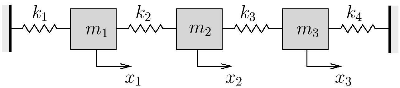
Consider the following cases:
i)

ii)

iii)

Note that the stiffness matrix for this problem is
![\[\bigl[ k \bigr] =\Biggl[\begin{array}{ccc}k_1 + k_2 & -k_2 & 0 \\-k_2 & k_2 + k_3 & -k_3 \\0 & -k_3 & k_3 + k_4 \\\end{array}\Biggr]\]](https://engcourses-uofa.ca/wp-content/ql-cache/quicklatex.com-273ee7a3ebd1314bec77497d4d9d116f_l3.png "Rendered by QuickLaTeX.com")
so that ![[a] = [k]^{-1}](https://engcourses-uofa.ca/wp-content/ql-cache/quicklatex.com-abdd102af30c73db144923944c6cc3d1_l3.png "Rendered by QuickLaTeX.com") is (Note: show full screen view)
is (Note: show full screen view)
![\[\bigl[ a \bigr] =\frac{1}{k_1 (k_2 k_3 + k_2 k_4 + k_3 k_4) + k_2 k_3 k_4}\Biggl[\begin{array}{ccc}k_2 k_3 + k_2 k_4 + k_3 k_4 & k_2\bigl( k_3 + k_4 \bigr) & k_2 k_3 \\k_2\bigl( k_3 + k_4 \bigr) & \bigl( k_1 + k_2 \bigr)\bigl( k_3 + k_4 \bigr) & \bigl( k_1 + k_2 \bigr)k_3 \\k_2 k_3 & \bigl( k_1 + k_2 \bigr)k_3 & k_1 k_2 + k_1 k_3 + k_2 k_3 \\\end{array}\Biggr]\]](https://engcourses-uofa.ca/wp-content/ql-cache/quicklatex.com-3adeb5d89acac11020ac93204792ffda_l3.png "Rendered by QuickLaTeX.com")
EXAMPLE
Use Dunkerley’s method to estimate the fundamental natural frequency for a light simply supported beam supporting three equally spaced identical masses.
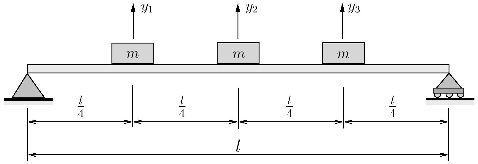
Note that for this system
![\begin{align*}\bigl[ a \bigr] =&\frac{l^3}{768 EI}\Biggl[\begin{array}{ccc}9 & 11 & 7\\11 & 16 & 11\\7 & 11 & 9\\\end{array}\Biggr] \\\bigl[ k \bigr] =&\frac{192 EI}{7 l^3}\Biggl[\begin{array}{rrr}23 & -22 & 9\\-22 & 32 & -22\\9 & -22 & 23\\\end{array}\Biggr] \\\bigl[ m \bigr] =&m\Biggl[\begin{array}{ccc}1 & 0 & 0\\0 & 1 & 0\\0 & 0 & 1\\\end{array}\Biggr] \\\end{align*}](https://engcourses-uofa.ca/wp-content/ql-cache/quicklatex.com-2d7b0dca2259bd0e7f15c8e14c292594_l3.png "Rendered by QuickLaTeX.com")
Dunkerley’s Formula to Estimate The Highest Natural Frequency
The ideas behind Dunkerley’s Formula, with a slightly different formulation, can also be used to estimate the highest natural frequency in a system. To see this start with (9.9)
![\begin{equation*}-\ensuremath{p}^2 \bigl[m\bigr]\!\bigl\{\!\mathbb{A}\!\bigr\} + \bigl[k\bigr]\!\bigl\{\!\mathbb{A}\!\bigr\} = \bigl\{0\bigr\}\end{equation*}](https://engcourses-uofa.ca/wp-content/ql-cache/quicklatex.com-3b5c265b9ee10e7a0418b152ebd7b9e3_l3.png "Rendered by QuickLaTeX.com")
Premultiplication by ![\bigl[m\bigr]\!\!\rule[5mm]{0pt}{0pt}^{-1}](https://engcourses-uofa.ca/wp-content/ql-cache/quicklatex.com-3812b0b0165debdfaea197bde3ed27b9_l3.png "Rendered by QuickLaTeX.com") produces
produces
![\begin{equation*}-\ensuremath{p}^2 \underbrace{\bigl[m\bigr]\!\!\rule[5mm]{0pt}{0pt}^{-1}\bigl[m\bigr]}_{\bigl[1\bigr]}\!\bigl\{\!\mathbb{A}\!\bigr\} + \bigl[m\bigr]\!\!\rule[5mm]{0pt}{0pt}^{-1}\bigl[k\bigr]\!\bigl\{\!\mathbb{A}\!\bigr\} = \bigl\{0\bigr\}\end{equation*}](https://engcourses-uofa.ca/wp-content/ql-cache/quicklatex.com-89496022c63a6804e360bbce2856d43f_l3.png "Rendered by QuickLaTeX.com")
or
![\begin{equation*}\biggl[\bigl[m\bigr]\!\!\rule[5mm]{0pt}{0pt}^{-1}\!\bigl[k\bigr]- \ensuremath{p}^2 \bigl[1\bigr] \biggr] \bigl\{\!\mathbb{A}\!\bigr\} = \bigl\{0\bigr\}\end{equation*}](https://engcourses-uofa.ca/wp-content/ql-cache/quicklatex.com-830ab30d6cc5ba5c02607064ddef56ae_l3.png "Rendered by QuickLaTeX.com")
This again requires, for non-trivial solutions,
(9.17) ![\begin{equation*}\biggl| \bigl[m\bigr]\!\!\rule[5mm]{0pt}{0pt}^{-1}\!\bigl[k\bigr]- \ensuremath{p}^2 \bigl[1\bigr] \biggr| = 0\end{equation*}](https://engcourses-uofa.ca/wp-content/ql-cache/quicklatex.com-cc7c00449eeb4be9801e77d103a1db13_l3.png "Rendered by QuickLaTeX.com")
If we again assume that the mass matrix is diagonal, then the inverse is simply
![\begin{equation*}\left[\begin{matrix}m_1 & 0 & \dots & 0 \\0 & m_2 & \dots & 0 \\\vdots & \vdots & \ddots & \vdots \\0 & 0 & \dots & m_N \\\end{matrix}\right]\!\!\!\rule[15mm]{0pt}{0pt}^{-1}=\left[\begin{matrix}\frac{1}{m_1} & 0 & \dots & 0 \\0 & \frac{1}{m_2} & \dots & 0 \\\vdots & \vdots & \ddots & \vdots \\0 & 0 & \dots & \frac{1}{m_N} \\\end{matrix}\right]\end{equation*}](https://engcourses-uofa.ca/wp-content/ql-cache/quicklatex.com-137842700abadeacc7f03d4f841aa6db_l3.png "Rendered by QuickLaTeX.com")
As a result, the determinant in (9.17) has the form
![\begin{equation*}\left| \left[\begin{matrix}\frac{1}{m_1} & 0 & \dots & 0 \\0 & \frac{1}{m_2} & \dots & 0 \\\vdots & \vdots & \ddots & \vdots \\0 & 0 & \dots & \frac{1}{m_N} \\\end{matrix}\right]\left[\begin{matrix}k_{{1}{1}} & k_{{1}{2}} & \dots & k_{{1}{N}} \\k_{{2}{1}} & k_{{2}{2}} & \dots & k_{{2}{N}} \\\vdots & \vdots & \ddots & \vdots \\k_{{N}{1}} & k_{{N}{2}} & \dots & k_{{N}{N}} \\\end{matrix}\right]-\left[\begin{matrix}\ensuremath{p}^2 & 0 & \dots & 0 \\0 & \ensuremath{p}^2 & \dots & 0 \\\vdots & \vdots & \ddots & \vdots \\0 & 0 & \dots & \ensuremath{p}^2 \\\end{matrix}\right] \right|= 0\end{equation*}](https://engcourses-uofa.ca/wp-content/ql-cache/quicklatex.com-6c068af66a52ff1108e06701675b9f6e_l3.png "Rendered by QuickLaTeX.com")
or
(9.18) ![\begin{equation*} \left|\begin{matrix}\Bigl(\dfrac{k_{{1}{1}}}{m_1} - p^2 \Bigr) & \dfrac{k_{{1}{2}}}{m_1} & \dots& \dfrac{k_{{1}{N}}}{m_1} \\[5mm]\dfrac{k_{{2}{1}}}{m_2} & \Bigl(\dfrac{k_{{2}{2}}}{m_2} - p^2\Bigr) & \dots &\dfrac{k_{{2}{N}}}{m_2} \\\vdots & \vdots & \ddots & \vdots \\\dfrac{k_{{N}{1}}}{m_N} & \dfrac{k_{{N}{2}}}{m_N} & \dots& \Bigl(\dfrac{k_{{N}{N}}}{m_N} - p^2\Bigr) \\\end{matrix}\right|= 0\end{equation*}](https://engcourses-uofa.ca/wp-content/ql-cache/quicklatex.com-f7c8d95b63c8c8ec1da543206bb7e1c7_l3.png "Rendered by QuickLaTeX.com")
Expanding (9.18) produces a characteristic equation with the form
(9.19) 
where  and
and  are again constants which depend on and
 ![\bigl[k\bigr]](https://engcourses-uofa.ca/wp-content/ql-cache/quicklatex.com-2aab9db82919d8134feae5242052b74d_l3.png "Rendered by QuickLaTeX.com") . The roots of (9.19) correspond to the natural frequencies of the system given by
. The roots of (9.19) correspond to the natural frequencies of the system given by

Once again, since these values are the roots of the characteristic equation, we could equivalently write the characteristic equation as
(9.20) 
which expanded gives
(9.21) 
where and are the same constants as in (9.19) Comparing the  terms in equations (9.19) and (9.21) shows that
(9.22) 
Since  is the largest natural frequency in the system, we ignore all of the other terms on the LHS of (9.22) to get

or more generally
(9.23) 
Due to the terms that have been ignored in (9.22), the frequency obtained using (9.23) will be larger than the highest natural frequency in the system. As a result, this version of Dunkerley’s Formula provides an upper bound on the largest natural frequency of the system.
EXAMPLE
For the system shown below:
(a) Use Rayleigh’s quotient to find an upper bound to the lowest natural frequency. Use a trial vector of

(b) Use Dunkerley’s method to find a lower bound for the lowest natural frequency.
(c) Use Dunkerley’s method to find an upper bound for the highest natural frequency.
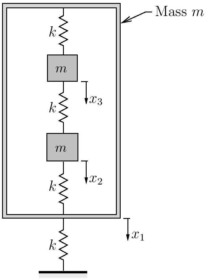
Note that for this problem,
![\begin{align*}\bigl[ k \bigr] =&k\Biggl[\begin{array}{rrr}3 & -1 & -1 \\-1 & 2 & -1 \\-1 & -1 & 2 \\\end{array}\Biggr] \\\bigl[ a \bigr] =&\frac{1}{3k}\Biggl[\begin{array}{rrr}3 & 3 & 3 \\3 & 5 & 4 \\3 & 4 & 5 \\\end{array}\Biggr] \\\bigl[ m \bigr] =&m\Biggl[\begin{array}{ccc}1 & 0 & 0\\0 & 1 & 0\\0 & 0 & 1\\\end{array}\Biggr] \\\end{align*}](https://engcourses-uofa.ca/wp-content/ql-cache/quicklatex.com-fab7604daffd835fda6d38cbefc6ad30_l3.png "Rendered by QuickLaTeX.com")