
Multiple Degree of Freedom Systems: Free Vibrations of Two Degree of Freedom Systems
Up to now, all of the systems that we have considered have been single degree of freedom systems for which one coordinate is sufficient to completely specify the configuration of the system. While there are numerous systems that can be reasonably modeled as having a single degree of freedom, there are many other systems that require a more detailed model.
Discrete vibrating systems are classified as either single degree of freedom (SDOF) or multiple degree of freedom (MDOF) systems. There are many parallels between single and multiple degree of freedom systems. We will begin our discussion of MDOF systems by considering two degree of freedom (TDOF) systems which are the simplest. This will help to illustrate all of the important features of MDOF systems while keeping the development as simple as possible. Once the two degree of freedom system is understood, extensions to systems with more degrees of freedom is straightforward.
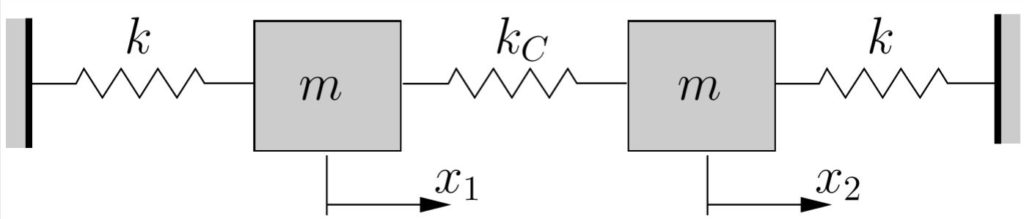
Consider a system comprised of two masses and several springs as shown in Figure 8.1. This is a two degree of freedom system since two coordinates are required to completely specify the configuration of the system. One set of coordinates which can be used is  and
and  , measured from the equilibrium position, as shown. However, this is not the only set of coordinates which could be used. In fact, while and seem like a natural and logical choice, in some sense there is a better choice, for reasons to be discussed shortly.
Preliminary Physical Reasoning
Before finding the actual solution to this problem, consider two specific initial displacements from the equilibrium configuration as shown in Figure 8.2 and see what we can deduce about the resulting motion. In Figure 8.2,  and
and  are the initial displacements of the two masses.
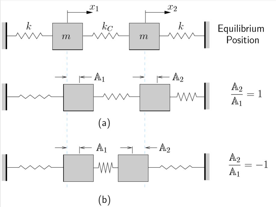
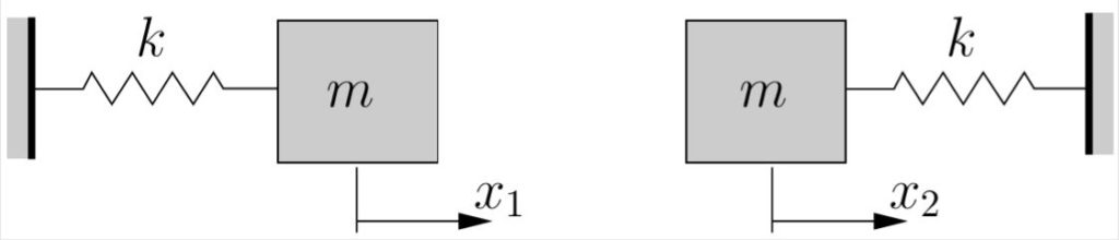
In case (a), both masses are displaced an equal amount in the same direction. In such a displacement, the central spring is neither stretched nor compressed (relative to its equilibrium length). Due to the symmetry in the system, both masses will undergo the same motion so that the distance between them will remain constant. The central spring remains completely undeformed in the resulting motion and applies no force on the masses. It therefore has no effect on the resulting motion (i.e. for this specific initial displacement, the motion of the system would be the same if the central spring were not present as shown in Figure 8.3.
As a result, we expect that if the masses are initially displaced with  and released from rest, the resulting motion would have
  and the oscillations would occur at a frequency of

In the second case (b), the masses are again displaced by equal amounts but in opposite directions. The central spring will extend and compress in this case. However, due to the symmetry in the system, the midpoint of the central spring remains stationary and does not move to the left or the right. As a result, the system behaves as if this were a fixed point, so that in this case we can think of the system as equivalent to that shown in Figure 8.4.
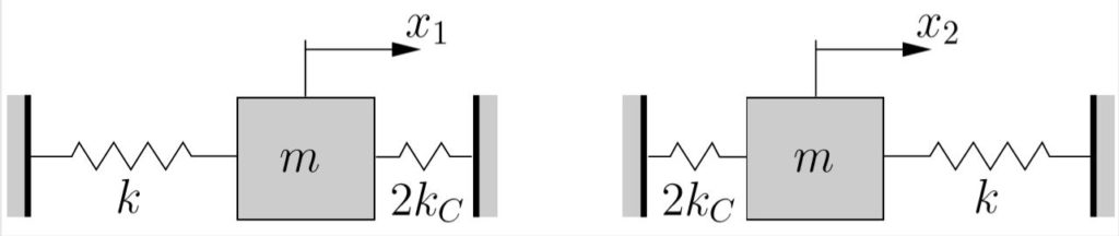
The fixed boundary in Figure 8.4 has the same effect on the system as the stationary central point. Since one half of the middle spring appears in each system, the effective spring constant in each system is  (remember that, other factors being equal, shorter springs are stiffer). Each mass in Figure 8.4 therefore is supported by two springs in parallel so the effective stiffness of each system is
  . As a result, we expect that if the masses are initially displaced with
  and released from rest, the resulting motion would be such that
  and the oscillations would occur at a frequency of

Equations of Motion
Having selected the coordinates ( and ) to describe the configuration of the system, the next step is to find the equations of motion in terms of the chosen coordinates (and their derivatives). Since this is a two degree of freedom system, we will get two equations of motion. There is usually one equation of motion per degree of freedom in the system. There are many ways to find these equations, and most of these methods are beyond the scope of this course. Here we will focus on the use of Newton’s Laws. As with single degree of freedom systems, when drawing FBD/MAD’s we generally assume that all of the coordinates and their derivatives are positive to get the correct signs in the equations of motion. To make things easier, you may also assume if you wish that one of the coordinates is larger than the other, say assume  , although it is not necessary to do so.
Figure 8.5 show the FBD/MAD for each of the masses in the system.
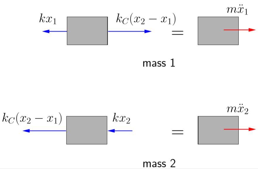
Applying Newtons law’s for mass 1 gives

while for mass 2 we get

so that the two equations of motion for the system are
(8.1a) 
(8.1b) 
It will be convenient to write these equations in matrix form, introducing the concept of mass and stiffness matrices, as
(8.2) ![\begin{equation*}\underbrace{\begin{bmatrix}m & 0 \\[1mm]0 & m \\\end{bmatrix}}_{\text{Mass Matrix}}\!\biggl\{\!\!\!\begin{array}{c}\ddot{x}_1 \\[1mm] \ddot{x}_2 \\\end{array}\!\!\!\biggr\}+\underbrace{\begin{bmatrix}k +k_C & -k_C \\[1mm]-k_C & k+k_C \\\end{bmatrix}}_{\text{Stiffness Matrix}}\!\biggl\{\!\!\!\begin{array}{c}x_1 \\[1mm] x_2 \\\end{array}\!\!\!\biggr\}=\biggl\{\!\!\!\begin{array}{c}0 \\[1mm] 0 \\\end{array}\!\!\!\biggr\}\end{equation*}](https://engcourses-uofa.ca/wp-content/ql-cache/quicklatex.com-a217e090b36a2a1670f398ca873182c7_l3.png "Rendered by QuickLaTeX.com")
An important feature of these equations is that they are coupled, meaning that both and appear in each of these equations. As a result it is not possible to solve either (8.1a) or (8.1b) independently. They must be solved as a pair.
Solution to Equations of Motion
To solve (8.2) we look for solutions in which both masses are undergoing harmonic motion at the same frequency (known as s simple simultaneous harmonic motion). We assume the motion of the masses is of the form

or
(8.3) 
where  and
and  are the amplitudes of motion of masses 1 and 2 respectively. With this assumption we see that

so the equations of motion become

![\begin{equation*}\Biggl[\begin{bmatrix}-m p^2 & 0 \\0 & -m p^2 \\\end{bmatrix}+\begin{bmatrix}k +k_C & -k_C \\-k_C & k+k_C \\\end{bmatrix}\Biggl]\biggl\{\!\!\!\begin{array}{c}\mathbb{A}_1 \\ \mathbb{A}_2 \\\end{array}\!\!\!\biggr\} \sin{(pt+\phi)}=\biggl\{\!\!\!\begin{array}{c}0 \\ 0 \\\end{array}\!\!\!\biggr\}\end{equation*}](https://engcourses-uofa.ca/wp-content/ql-cache/quicklatex.com-9248451b9557ede98282caff4d9a779e_l3.png "Rendered by QuickLaTeX.com")
or

which must be satisfied at all times  . The only way this can be true is if
(8.4) 
There are two possibilities:
(i) 
This implies that there is no motion (see equation (8.3)). This is called the trivial solution and is not of interest here.
(ii) The determinant  is equal to zero.
This is a result from linear algebra and is required for equation (8.4) to have a non-trivial solution.
For a  matrix
  , the determinant is
  so
so

or

or
(8.5) 
This is known as the characteristic equation for this system and can be seen to be a quadratic equation for  .
.
The two roots are

![\[= \frac{\frac{\cancel{2}(k+k_C)}{m} \pm \frac{\cancel{2}}{m}\sqrt{\cancel{k^2} + \cancel{2kk_C} + k_C^2 - \cancel{k^2} - \cancel{2kk_C}}}{\cancel{2}}\]](https://engcourses-uofa.ca/wp-content/ql-cache/quicklatex.com-0dda3fc5c46577f99263115ac54550ff_l3.png "Rendered by QuickLaTeX.com")

(8.6) 
Equation (8.6) gives us the two natural frequencies for our two degrees of freedom system. While the numbering of these frequencies is essentially arbitrary, it is customary to number them from lowest to highest. Therefore  is understood to be lowest natural frequency of the system. This is also referred to as the fundamental natural frequency. These natural frequencies agree with those expected based on our earlier preliminary physical reasoning. When the system is vibrating at one of these frequencies, we say that it is vibrating in one of its modes. A two degree of freedom system will therefore have two modes of vibration.
Note that for our two degree of freedom system we obtained a second order polynomial (quadratic) characteristic equation from which we have found two natural frequencies. In general, if we have an  degree of freedom system, we will find equations of motion. The solution of these leads to an
  order polynomial characteristic equation from which we can find natural frequencies.
Having found the natural frequencies, we would like to determine the amplitudes and that occur in each mode. To do so we again consider equation (8.4)

Since we have now found the two natural frequencies, we can use these in turn to find and . However, we cannot simply substitute the values of from (8.6) into ) into equation (8.4) and solve for and due to the fact that the matrix is singular for these two values of (that was the condition we used to find these natural frequencies originally).
Since the square matrix equation (8.4) will be singular, we cannot solve for and uniquely. However, we can find a ratio between and for each . To see this, consider the first natural frequency  . Substituting this value into equation (8.4) gives
![\begin{equation*}\begin{align}\begin{bmatrix}k + k_C - m\left(\frac{k}{m}\right) & -k_C \\- k_C & k + k_C - m\left(\frac{k}{m}\right)\end{bmatrix}\!\!\biggl\{\!\!\!\begin{array}{c}\mathbb{A}_1 \\ \mathbb{A}_2 \\\end{array}\!\!\!\biggr\}& =\biggl\{\!\!\!\begin{array}{c}0 \\ 0 \\\end{array}\!\!\!\biggr\} \\[2mm]\begin{bmatrix}k_C & -k_C \\- k_C & k_C\end{bmatrix}\!\!\biggl\{\!\!\!\begin{array}{c}\mathbb{A}_1 \\ \mathbb{A}_2 \\\end{array}\!\!\!\biggr\}& =\biggl\{\!\!\!\begin{array}{c}0 \\ 0 \\\end{array}\!\!\!\biggr\}\end{align}\end{equation}](https://engcourses-uofa.ca/wp-content/ql-cache/quicklatex.com-5ac6065bce1082842b400940f62aaa2d_l3.png "Rendered by QuickLaTeX.com")
The first of these equations gives

or
(8.7) 
Similarly, the second gives

or, once again

which shows that it does not matter which of the equations in (8.4) is used.
Now consider the second natural frequency  . Substituting this result into equation (8.4) gives
![\begin{equation*}\begin{align}\begin{bmatrix}k + k_C - m\left(\frac{k+2k_C}{m}\right) & -k_C \\- k_C & k + k_C - m\left(\frac{k+2k_C}{m}\right)\end{bmatrix}\!\!\biggl\{\!\!\!\begin{array}{c}\mathbb{A}_1 \\ \mathbb{A}_2 \\\end{array}\!\!\!\biggr\}& =\biggl\{\!\!\!\begin{array}{c}0 \\ 0 \\\end{array}\!\!\!\biggr\} \\[2mm]\begin{bmatrix}-k_C & -k_C \\- k_C & -k_C\end{bmatrix}\!\!\biggl\{\!\!\!\begin{array}{c}\mathbb{A}_1 \\ \mathbb{A}_2 \\\end{array}\!\!\!\biggr\}& =\biggl\{\!\!\!\begin{array}{c}0 \\ 0 \\\end{array}\!\!\!\biggr\}\end{align}\end{equation}](https://engcourses-uofa.ca/wp-content/ql-cache/quicklatex.com-61bef35a0af576e1b2f70d2380e69cce_l3.png "Rendered by QuickLaTeX.com")
The first of these equations gives

or
(8.8) 
The second equation gives
or

as before.
Therefore as we can see, there is a particular ratio of the amplitudes of motion of the two masses when they are vibrating at one of the system’s natural frequencies. We have also shown that either of the equations in equation (8.4) can be used to determine this amplitude ratio.
In summary, we have shown that for this system
(8.9) 
(8.10) 
The terms
(8.11) 
represent the ratio of the amplitudes of the masses when they execute simple simultaneous harmonic motion at the first and second natural frequencies respectively. These do not determine the values of and uniquely, only their ratio. To use this information effectively, typically one of the amplitudes in the system is arbitrarily assigned a value of 1. The magnitude of the other amplitude can then be uniquely determined using the appropriate ratio. For example, if we arbitrarily assign  , then we see from equation (8.9) that for ,

For the second natural frequency (i.e. in the second mode), equation (8.10) gives

We can represent these results as
(8.12) 
With these results, the response of the system in each of the first and second modes as given in equation (8.3) can be written as
![\begin{equation*}\biggl\{\!\!\!\begin{array}{c}x_1(t) \\ x_2(t) \\\end{array}\!\!\!\biggr\}=\biggl\{\!\!\!\begin{array}{r}\mathbb{A}_1 \\ \mathbb{A}_2 \\\end{array}\!\!\!\biggr\}^{\textcircled{{\footnotesize{1}}}} \, \Bigl[ \sin{(p_1 t + \phi_1)} \Bigr]\end{equation*}](https://engcourses-uofa.ca/wp-content/ql-cache/quicklatex.com-c0f96ddfd4acdf1765585cdc2facfaa3_l3.png "Rendered by QuickLaTeX.com")
and
![\begin{equation*}\biggl\{\!\!\!\begin{array}{c}x_1(t) \\ x_2(t) \\\end{array}\!\!\!\biggr\}=\biggl\{\!\!\!\begin{array}{r}\mathbb{A}_1 \\ \mathbb{A}_2 \\\end{array}\!\!\!\biggr\}^{\textcircled{{\footnotesize{2}}}} \, \Bigl[ \sin{(p_2 t + \phi_2)} \Bigr]\end{equation*}](https://engcourses-uofa.ca/wp-content/ql-cache/quicklatex.com-c8943ac9f10c0877897bd388d6720b33_l3.png "Rendered by QuickLaTeX.com")
The terms
(8.13) 
are known as the first and second mode shapes respectively. These are also referred to as the normal modes of the system. Often, these mode shapes are normalized so that they represent a unit vector. We could then equivalently write them as

As we have seen there are several ways that the mode shapes can be expressed. Each of these is correct, although in this course we will most often use the form in equation (8.12). What is important is that that the ratio of the amplitudes in any given mode is as given in equations (8.7) and (8.8).
EXAMPLE
The double pulley shown below (which is supported by a spring with stiffness  ) has a moment of inertia
  about its center
  . The pulley supports a mass
  by a light cable which has an effective stiffness
  . The coordinates
  and
and  as shown are used to describe the system.
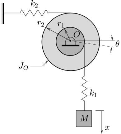
(a) Determine the equations of motion for this system using Newton’s Law’s.
(b) If

the equations of motion become

Determine the resulting natural frequencies for this system and sketch the associated mode shapes.
EXAMPLE
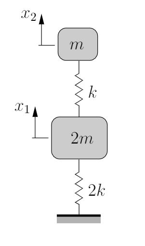
Determine expressions for the natural frequencies and mode shapes for the system shown. Use the coordinates and as indicated.
Response in Terms of Normal Modes
Normal modes can be used to conveniently express the response of the system. We have found two natural frequencies which each satisfy the equations of motion. For each of these frequencies there is an associated mode shape. Since the governing differential equations (8.2) are linear, the total solution can be expressed as a superposition of these two solutions
(8.14) ![\begin{align*}\biggl\{\!\!\!\begin{array}{c}x_1(t) \\ x_2(t) \\\end{array}\!\!\!\biggr\}&=\biggl\{\!\!\!\begin{array}{r}\mathbb{A}_1 \\ \mathbb{A}_2 \\\end{array}\!\!\!\biggr\}^{\textcircled{{\footnotesize{1}}}} \, \Bigl[ \sin{(p_1 t + \phi_1)} \Bigr] +\biggl\{\!\!\!\begin{array}{r}\mathbb{A}_1 \\ \mathbb{A}_2 \\\end{array}\!\!\!\biggr\}^{\textcircled{{\footnotesize{2}}}} \, \Bigl[ \sin{p_2 t + \phi_2} \Bigr] \nonumber \\\intertext{or}\biggl\{\!\!\!\begin{array}{c}x_1(t) \\ x_2(t) \\\end{array}\!\!\!\biggr\}&=\mathbb{A}_1^{\textcircled{{\footnotesize{1}}}}\underbrace{\biggl\{\!\!\!\begin{array}{r}1 \\ 1 \\\end{array}\!\!\!\biggr\} \, \sin{(p_1 t + \phi_1)}}_{\text{First Mode Response}} +\mathbb{A}_1^{\textcircled{{\footnotesize{2}}}}\underbrace{\biggl\{\!\!\!\begin{array}{r}1 \\ -1 \\\end{array}\!\!\!\biggr\} \, \sin{(p_2 t + \phi_2)}}_{\text{Second Mode Response}}\label{eq:8.14}\end{align*}](https://engcourses-uofa.ca/wp-content/ql-cache/quicklatex.com-41417af56abb9ef9ec34825a79309084_l3.png "Rendered by QuickLaTeX.com")
where  and
and  represent the actual amplitude of the motion of mass 1 in the first and second modes respectively, which will depend on the initial conditions as we will discuss shortly. Note that equation (8.14) simply represents two equations

where

It can be verified by direct substitution that these equations are indeed the solutions to the equations of motion.
There are four arbitrary constants in the solution:  and
and  . The (scalar) quantities and represent how much of each mode is present in the response while
  and represent the relative phase angle of each of the modes. Note that the equations in (8.14) can be rewritten as
![\begin{align*}\biggl\{\!\!\!\begin{array}{c}x_1(t) \\ x_2(t) \\\end{array}\!\!\!\biggr\}&=\mathbb{A}_1^{\textcircled{{\footnotesize{1}}}}\biggl\{\!\!\!\begin{array}{r}1 \\ 1 \\\end{array}\!\!\!\biggr\} \, \Bigl[ \sin{(p_1 t + \phi_1)} \Bigr] +\mathbb{A}_1^{\textcircled{{\footnotesize{2}}}}\biggl\{\!\!\!\begin{array}{r}1 \\ -1 \\\end{array}\!\!\!\biggr\} \, \Bigl[ \sin{(p_2 t + \phi_2)} \Bigr] \nonumber \\[2mm]\biggl\{\!\!\!\begin{array}{c}x_1(t) \\ x_2(t) \\\end{array}\!\!\!\biggr\}&=\biggl\{\!\!\!\begin{array}{r}1 \\ 1 \\\end{array}\!\!\!\biggr\} \, \Bigl[\mathbb{A}_1^{\textcircled{{\footnotesize{1}}}} \sin{(p_1 t + \phi_1)} \Bigr] +\biggl\{\!\!\!\begin{array}{r}1 \\ -1 \\\end{array}\!\!\!\biggr\} \, \Bigl[\mathbb{A}_1^{\textcircled{{\footnotesize{2}}}} \sin{(p_2 t + \phi_2)} \Bigr] \nonumber \\\end{align}](https://engcourses-uofa.ca/wp-content/ql-cache/quicklatex.com-6a7c0c79de46e20341a8e998c1e1363a_l3.png "Rendered by QuickLaTeX.com")
or equivalently as
(8.15) ![\begin{align*}\label{eq:8.15}\biggl\{\!\!\!\begin{array}{c}x_1(t) \\ x_2(t) \\\end{array}\!\!\!\biggr\}&=\biggl\{\!\!\!\begin{array}{r}1 \\ 1 \\\end{array}\!\!\!\biggr\} \, \Bigl[ A \sin{(p_1 t)} + B \cos{(p_1 t)} \Bigr]+\biggl\{\!\!\!\begin{array}{r}1 \\ -1 \\\end{array}\!\!\!\biggr\} \, \Bigl[ C \sin{(p_2 t)} + D \cos{(p_2 t)} \Bigr]\end{align*}](https://engcourses-uofa.ca/wp-content/ql-cache/quicklatex.com-4275a4dd253e6ce1a5dfa1cd021255f0_l3.png "Rendered by QuickLaTeX.com")
where  and
and  are now the four arbitrary constants. These quantities are determined by the initial conditions. With four arbitrary constants, we will need four initial conditions to determine them uniquely. The initial conditions used are typically the initial position and velocity of each of the masses. If for example

equation (8.15) at  becomes
![\begin{equation*}\biggl\{\!\!\!\begin{array}{c}x_{1_0} \\ x_{2_0} \\\end{array}\!\!\!\biggr\}=\biggl\{\!\!\!\begin{array}{r}1 \\ 1 \\\end{array}\!\!\!\biggr\} \, \Bigl[ B \Bigr]+\biggl\{\!\!\!\begin{array}{r}1 \\ -1 \\\end{array}\!\!\!\biggr\} \,\Bigl[ D \Bigr]\end{equation*}](https://engcourses-uofa.ca/wp-content/ql-cache/quicklatex.com-1aed9a18799642e2c74bdeb3ddcbdeab_l3.png "Rendered by QuickLaTeX.com")
so that

(8.16) ![\begin{equation*}\begin{split}\label{eq:8.16}B &= \frac{x_{1_0}+x_{2_0}}{2} \\[2mm]D &= \frac{x_{1_0}-x_{2_0}}{2}\end{split}\end{equation*}](https://engcourses-uofa.ca/wp-content/ql-cache/quicklatex.com-00f9a2c2fdd7c6b1f34f73632940aa6b_l3.png "Rendered by QuickLaTeX.com")
Differentiating {8.15}
![\begin{equation*}\biggl\{\!\!\!\begin{array}{c}\dot{x}_1(t) \\ \dot{x}_2(t) \\\end{array}\!\!\!\biggr\}=\biggl\{\!\!\!\begin{array}{r}1 \\ 1 \\\end{array}\!\!\!\biggr\} \, \Bigl[ A p_1 \cos{(p_1 t)} - B p_1 \sin{(p_1 t)} \Bigr]+\biggl\{\!\!\!\begin{array}{r}1 \\ -1 \\\end{array}\!\!\!\biggr\} \, \Bigl[ C p_2 \cos{(p_2 t)} - D p_2 \sin{(p_2 t)} \Bigr]\end{equation*}](https://engcourses-uofa.ca/wp-content/ql-cache/quicklatex.com-46a81fd646956cb8f23c0be4f25c5d2e_l3.png "Rendered by QuickLaTeX.com")
and substituting the above initial conditions leads to
![\begin{equation*}\biggl\{\!\!\!\begin{array}{c}v_{1_0} \\ v_{2_0} \\\end{array}\!\!\!\biggr\}=\biggl\{\!\!\!\begin{array}{r}1 \\ 1 \\\end{array}\!\!\!\biggr\} \, \Bigl[ A p_1 \Bigr]+\biggl\{\!\!\!\begin{array}{r}1 \\ -1 \\\end{array}\!\!\!\biggr\} \,\Bigl[ C p_2 \Bigr]\end{equation*}](https://engcourses-uofa.ca/wp-content/ql-cache/quicklatex.com-85e8a5f48cef5d9f370583097bbf87f0_l3.png "Rendered by QuickLaTeX.com")
so that

which can again be solved to find
(8.17) ![\begin{equation*}\begin{split}\label{eq:8.17}A &= \frac{v_{1_0}+v_{2_0}}{2p_1} \\[2mm]C &= \frac{v_{1_0}-v_{2_0}}{2p_2}\end{split}\end{equation*}](https://engcourses-uofa.ca/wp-content/ql-cache/quicklatex.com-324760c3ff323cb6a924f775febe03c9_l3.png "Rendered by QuickLaTeX.com")
As a result, the total response then becomes
(8.18) ![\begin{equation*}\begin{split}\label{eq:8.18}\biggl\{\!\!\!\begin{array}{c}x_1(t) \\ x_2(t) \\\end{array}\!\!\!\biggr\}=\biggl\{\!\!\!\begin{array}{r}1 \\ 1 \\\end{array}\!\!\!\biggr\} \, &\biggl[\Bigl( \frac{v_{1_0}+v_{2_0}}{2p_1}\Bigr) \sin{(p_1 t)} +\Bigl( \frac{x_{1_0}+x_{2_0}}{2} \Bigr) \cos{(p_1 t)} \biggr]+\\\biggl\{\!\!\!\begin{array}{r}1 \\ -1 \\\end{array}\!\!\!\biggr\} \, &\biggl[\Bigl( \frac{v_{1_0}-v_{2_0}}{2p_2}\Bigr) \sin{(p_2 t)} +\Bigl( \frac{x_{1_0}-x_{2_0}}{2} \Bigr) \cos{(p_2 t)} \biggr]\end{split}\end{equation*}](https://engcourses-uofa.ca/wp-content/ql-cache/quicklatex.com-db3f29e075c1f5f3bd7bbddd5cd09d8d_l3.png "Rendered by QuickLaTeX.com")
If equation (8.14} was to be used then note that
![\begin{align*}A_1^{\textcircled{{\footnotesize{1}}}} &=\sqrt{ \Bigl[ \frac{v_{1_0}+v_{2_0}}{2p_1} \Bigr]^2 +\Bigl[ \frac{x_{1_0}+x_{2_0}}{2}\Bigr]^2},\qquad &\phi_1 &= \arctan\Biggl[ \frac{x_{1_0}+x_{2_0}}{\frac{v_{1_0}+v_{2_0}}{2p_1}}\Biggr ] \\[2mm]A_1^{\textcircled{{\footnotesize{2}}}} &=\sqrt{ \Bigl[ \frac{v_{1_0}-v_{2_0}}{2p_2} \Bigr]^2 +\Bigl[ \frac{x_{1_0}-x_{2_0}}{2}\Bigr]^2}, &\phi_2 &= \arctan\Biggl[ \frac{x_{1_0}-x_{2_0}}{\frac{v_{1_0}-v_{2_0}}{2p_2}}\Biggr ]\end{align*}](https://engcourses-uofa.ca/wp-content/ql-cache/quicklatex.com-9b4f3b265232bd4f47fbcdb9c59c8986_l3.png "Rendered by QuickLaTeX.com")
To see how we can use these results, consider the two specific sets of initial conditions considered previously:
(i) Both masses displaced the same amount  in the same direction and released from rest. The associated initial conditions are

The response from (8.18) is then
![\begin{equation*}\biggl\{\!\!\!\begin{array}{c}x_1(t) \\ x_2(t) \\\end{array}\!\!\!\biggr\}=\biggl\{\!\!\!\begin{array}{r}1 \\ 1 \\\end{array}\!\!\!\biggr\} \, \Bigl[ x_0 \cos{(p_1 t)} \Bigr]\end{equation*}](https://engcourses-uofa.ca/wp-content/ql-cache/quicklatex.com-a4c9af4e32e0133f396b6de081167979_l3.png "Rendered by QuickLaTeX.com")
which shows that the response of the system is entirely in the first mode. The masses move together at the same frequency () with the same amplitude in the same direction  at all times. In this motion the middle spring remains undeformed.
(ii) Both masses displaced the same amount in opposite directions and released from rest. The associated initial conditions are

The response from (8.18) is then
![\begin{equation*}\biggl\{\!\!\!\begin{array}{c}x_1(t) \\ x_2(t) \\\end{array}\!\!\!\biggr\}=\biggl\{\!\!\!\begin{array}{r}1 \\ -1 \\\end{array}\!\!\!\biggr\} \, \Bigl[ x_0 \cos{(p_2 t)} \Bigr]\end{equation*}](https://engcourses-uofa.ca/wp-content/ql-cache/quicklatex.com-ad3ead21bb25b65d02c8712dabe0f83f_l3.png "Rendered by QuickLaTeX.com")
which shows that now the response of the system is entirely in the second mode. The masses again move with the same amplitude and the same frequency ( ) but in opposite directions
  at all times. In this motion the midpoint of the central spring does not move.
This highlights a general result, but a very important one. The response of a multiple degree of freedom linear system will always be a linear combination of the normal mode responses of the system, with each mode responding at its associated natural frequency. The amount (amplitude) of each mode and the corresponding phase angle are determined solely by the initial conditions. This is the fundamental idea behind the approach known as modal analysis. As we have seen above, if a system is started in one of its modes (both position and velocity must satisfy these conditions) then it will vibrate purely in that mode. If the initial conditions do not start the system in one of its modes, then the response will in general be a combination of the modes in the system.
These results completely agree with (and generalize) the previous results we predicted for certain special situations based on purely physical reasoning. Of course, the mathematical approach outlined here will usually be required when the systems become more complex.
Beating
Beating is a phenomenon that occurs in MDOF systems when natural frequencies are “close” to each other. To see this, consider the simple two degree of freedom system we have been investigating with initial conditions such that only one mass is displaced from the equilibrium position and released from rest

With these initial conditions we find from (8.16) and (8.17) that

so the response will be
![\begin{equation*}\biggl\{\!\!\!\begin{array}{c}x_1(t) \\ x_2(t) \\\end{array}\!\!\!\biggr\}=\biggl\{\!\!\!\begin{array}{r}1 \\ 1 \\\end{array}\!\!\!\biggr\} \, \biggl[\frac{\mathbb{X}}{2} \cos{(p_1 t)}\biggr] +\biggl\{\!\!\!\begin{array}{r}1 \\ -1 \\\end{array}\!\!\!\biggr\} \, \biggl[\frac{\mathbb{X}}{2} \cos{(p_2 t)}\biggr]\end{equation*}](https://engcourses-uofa.ca/wp-content/ql-cache/quicklatex.com-65c9cdefab997f03bfb4cfd2df261cb0_l3.png "Rendered by QuickLaTeX.com")
or
![\begin{equation*}\begin{split}x_1(t) &= \frac{\mathbb{X}}{2}\Bigl[ \cos{(p_1 t)} + \cos{(p_2 t)} \Bigr] \\[2mm]x_2(t) &= \frac{\mathbb{X}}{2}\Bigl[ \cos{(p_1 t)} - \cos{(p_2 t)} \Bigr] \\\end{split}\end{equation*}](https://engcourses-uofa.ca/wp-content/ql-cache/quicklatex.com-94edf2da8f8995da21685d8895ebc1a6_l3.png "Rendered by QuickLaTeX.com")
Using appropriate trigonometric identities, these can equivalently be rewritten
(8.19) ![\begin{equation*}\label{eq:8.19}\begin{split}x_1(t) &= \mathbb{X} \cos \Bigl( \frac{(p_2-p_1)}{2} t \Bigr)\cos \Bigl( \frac{p_2+p_1}{2} t \Bigr) \\[2mm]x_2(t) &= \mathbb{X} \sin \Bigl( \frac{p_2-p_1}{2} t \Bigr)\sin \Bigl( \frac{p_2+p_1}{2} t \Bigr)\\\end{split}\end{equation*}](https://engcourses-uofa.ca/wp-content/ql-cache/quicklatex.com-806c4d25e5abfa3b52e292c6eee56be1_l3.png "Rendered by QuickLaTeX.com")
If we define

(8.19) becomes
![\begin{equation*}\begin{split}x_1(t) &= \Bigl[ \mathbb{X} \cos(\Delta t) \Bigr] \cos \Bigl( \frac{p_2+p_1}{2} t \Bigr) \\[2mm]x_2(t) &= \Bigl[ \mathbb{X} \sin(\Delta t) \Bigr] \sin \Bigl( \frac{p_2+p_1}{2} t \Bigr) \\\end{split}\end{equation*}](https://engcourses-uofa.ca/wp-content/ql-cache/quicklatex.com-b4932b0f77ce3afb64f31254ab1b7829_l3.png "Rendered by QuickLaTeX.com")
Now, if the two natural frequencies are close to each other, we can interpret these motions as vibrations occurring at a frequency of  with an amplitude that varies slowly at a frequency
  . We can define the beating frequency as

and the associated beating period as

Figure 8.6 illustrates this response of the two masses with

so that in this case

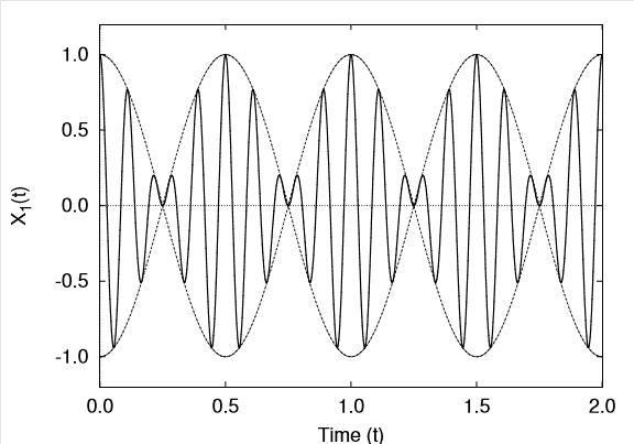
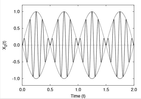
Note that in the beating response, there is a transfer of energy between the two masses. As can be seen in Figure (8.6), when mass 1 is vibrating with a maximum amplitude, the amplitude of mass 2 is small so that mass 1 has a large kinetic energy while mass 2 has almost none. One half of a beating period later the situation is reversed and mass 2 will have a large kinetic energy while mass 1 will have very little. Note further that since the system under consideration is conservative, the total mechanical energy remains constant at all times .
EXAMPLE
Two simple pendulums of the same length are connected by a light spring with stiffness  as shown.
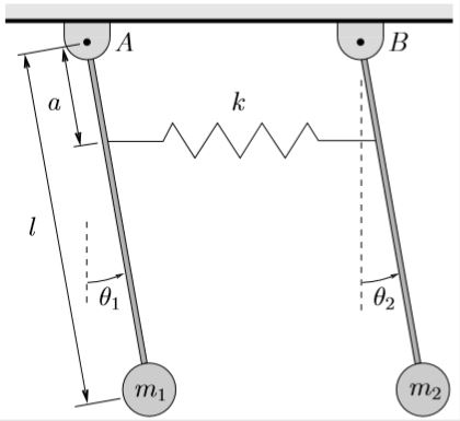
For this system, determine
(a) the equations of motion
(b) the natural frequencies
(c) the mode shapes
(d) the total response of the system (for  ) if the initial conditions at time are

For parts (b)–(d) assume that  .
.
nice good example