Sound and Acoustics: Frequency Analysis of Noise

To understand and quantify noise, we need to know about both the pressure levels involved as well as the frequency characteristics. The frequency is important for a number of reasons:

• Human hearing is frequency dependent. A noise with a certain sound pressure level at one frequency does not necessarily sound as loud as another noise with the same sound pressure level at a different frequency. Weighting scales have been developed to try to take these differences into account.
• Largely as a result of the above, many codes and regulations are expressed in terms of specific frequencies.

The human hearing range is between approximately 20 HZ and 20 000 HZ. As opposed to the decibel (logarithmic) scale used when dealing with sound pressures, a geometric scale is typically used when dealing with frequencies. In this approach, the audio spectrum is broken down into a number of convenient bands and the acoustic energy in each band is used. There are many types of frequency bands, but they share some common features.

Frequency Bands

A frequency band is defined by a lower frequency () and an upper frequency (). The bandwidth associated with a particular frequency band is simply the difference between the upper and lower frequencies

(12.43)  

Each band is typically named after its \emph{center} frequency which is defined as

(12.44)  

Note that this isn’t the average of the upper and lower frequencies but is the geometric mean with the property that

In absolute terms, is closer to than to , however, the term center frequency is commonly used.

The relationship between the upper and lower frequencies for each band follows a common rule, typically

(12.45)  

where the value of determines the type of band used. More generally, for the band

(12.46)  

This is illustrated for four bands schematically in 12.10.

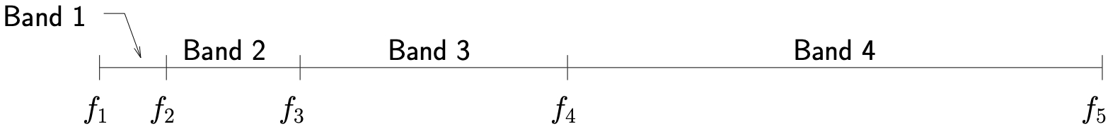
Figure 12.10: Illustration of relationship between bands and frequencies

As a result, the center frequency for each band becomes

so that

(12.47)  

Similarly we find that

(12.48)  

Therefore, the bandwidth is

(12.49)  

As can be seen, for a given , the bandwidth for any given band is a fixed percentage of the center frequency for that band. As a result, these types of bands are often referred to as percentage bands.

There are also systems which break up the frequency spectrum into bands with constant bandwidth. These are known as narrow bands. FFT analyzers fall into this category. These approaches are however not yet as standardized as the percentage band approach.

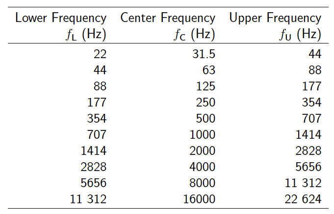
Table 12.5: Standard Octave Bands

Octave Bands

If in 12.45, then

so that the upper frequency is twice the lower one. These bands are known as octave bands. We also find from 12.49 that

so that the bandwidth is approximately 71% of the center frequency.

Most work with octave bands uses a standardized set of bands which are shown in Table 12.5. Note once again that each band is typically named after its center frequency, so we could talk about the 1000 HZ band, for example, which would include all frequencies between 707 and 1414 HZ. Characterizing noise in terms of octave bands is the crudest form of analysis. More refinement can be obtained by using fractional octave bands.

One-Third Octave Bands

For one-third octave bands, we set in 12.45 so that

so that the upper frequency is only 26\% larger than the lower. In terms of the center frequency we find that

so that the bandwidth is

which is approximately 23% of the center frequency. The standard one-third octave bands commonly used are shown in Table 12.6.

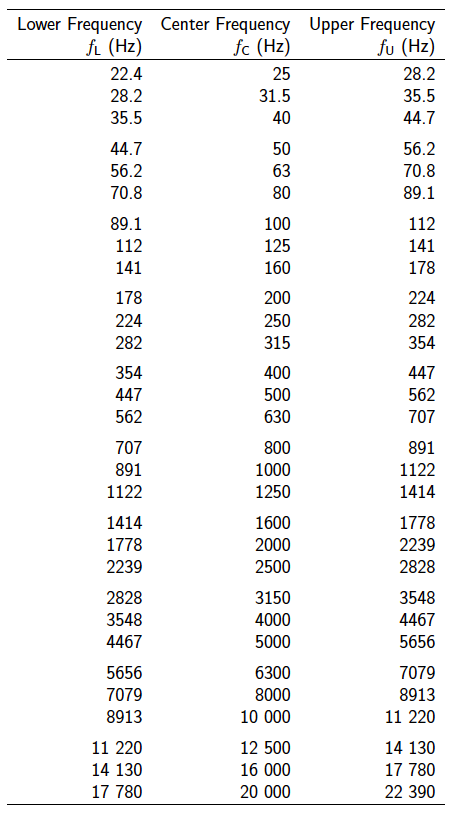
Table 12.6: Standard One-Third Octave Bands

Example

The octave band sound pressure levels for a centrifugal fan measured at 3~m are shown below.

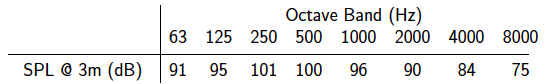
1. Determine the overall noise level (SPL) at 3 m.
2. Estimate the acoustic power of the fan. Assume that
   a) The fan is acting as a point source and acoustic energy is being radiated in all directions equally.
   b) The fan is located in the middle of a smooth floor which does not absorb any of the acoustic energy.