
Vibrations of Continuous Systems: Lateral Vibrations of Beams
Equation of Motion
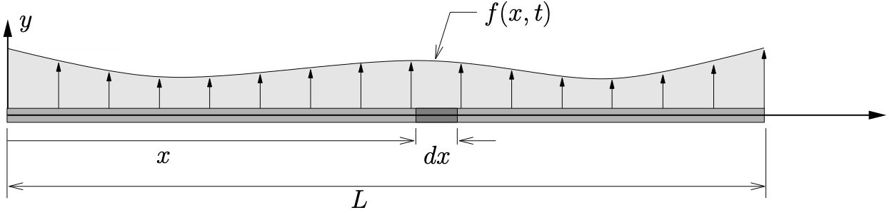
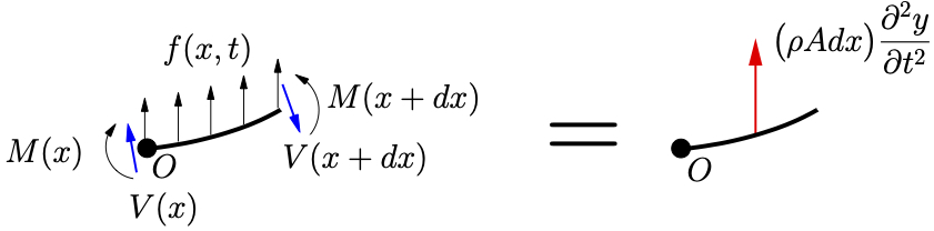
Figure 10.6: Uniform beam undergoing lateral vibrations
Consider a beam, shown in Figure 10.6(a) which has a length  , density
  (mass per unit volume) and Young’s modulus
  which is acted upon by a distributed load
  (per unit length) acting laterally along the beam. Let
  measure the lateral deflection of the beam and assume that only small deformations occur. Figure 10.6(b) shows the FBD/MAD for an infinitesimal element of the beam with mass
  . By applying Newton’s Law’s and considering moments about the left end of the element we find
![\begin{equation*}{\circlearrowleft}\Bigl[\sum M_O\Bigr]_{\text{FDB}} = \Bigl[\sum M_O\Bigr]_{\text{MAD}}\end{equation*}](https://engcourses-uofa.ca/wp-content/ql-cache/quicklatex.com-8376fa131c6a53677b82dc061c0d1751_l3.png "Rendered by QuickLaTeX.com")
![\[M(x+dx) - M(x) - V(x+dx) dx + \cancelto{}{f(x,t) dx \frac{dx}{2}} =\cancelto{2nd \quad order}{{dm \ensuremath{\frac{\partial^2 y}{\partial t^2}} \frac{dx}{2}}}}\]](https://engcourses-uofa.ca/wp-content/ql-cache/quicklatex.com-ca90721ebb1e9daadd389e0a3ac4030c_l3.png "Rendered by QuickLaTeX.com")
As a first order approximation we can write that
![\begin{align*}M(x+dx) &= M(x) + \frac{\partial M}{\partial x} dx \\[2mm]V(x+dx) &= V(x) + \frac{\partial V}{\partial x} dx \\\end{align*}](https://engcourses-uofa.ca/wp-content/ql-cache/quicklatex.com-9d0d6fc0da5d8b3dd08deca92716c163_l3.png "Rendered by QuickLaTeX.com")
so that the above becomes
![\[\Bigl[\cancel{M(x)} + \frac{\partial M}{\partial x} dx\Bigr] - \cancel{M(x)} -\Bigl[V(x) + \frac{\partial V}{\partial x} dx\Bigr] dx &= 0\]](https://engcourses-uofa.ca/wp-content/ql-cache/quicklatex.com-1c1ca08bf9e103b499e88c65281a0e22_l3.png "Rendered by QuickLaTeX.com")
![\[\frac{\partial M}{\partial x} dx - V(x) dx - \cancelto{small}{\frac{\partial V}{\partial x} dx }}dx &= 0\]](https://engcourses-uofa.ca/wp-content/ql-cache/quicklatex.com-2aacfd5da2c3dccdef9a32873028a6df_l3.png "Rendered by QuickLaTeX.com")
![\[\frac{\partial M}{\partial x} \cancel{dx} - V(x) \cancel{dx} = 0\]](https://engcourses-uofa.ca/wp-content/ql-cache/quicklatex.com-438315d8b2b9cde1e916408bb999025b_l3.png "Rendered by QuickLaTeX.com")
or
(10.23) 
which is a well known result from beam theory. In the vertical direction we then have
![\begin{align*}+\!\!\uparrow\sum F = ma:\qquadV(x) - V(x+dx) + f(x,t) dx &= \rho A dx \ensuremath{\frac{\partial^2 y}{\partial t^2}} \\{V(x)} - \Bigl[{V(x)} + \frac{\partial V}{\partial x} dx\Bigr]+ f(x,t) dx &= \rho A dx \ensuremath{\frac{\partial^2 y}{\partial t^2}} \\-\frac{\partial V}{\partial x} {dx} + f(x,t) {dx} &= \rho A {dx} \ensuremath{\frac{\partial^2 y}{\partial t^2}} \\\intertext{or}-\frac{\partial V}{\partial x} + f(x,t) &= \rho A \ensuremath{\frac{\partial^2 y}{\partial t^2}} \\\end{align*}](https://engcourses-uofa.ca/wp-content/ql-cache/quicklatex.com-ae188845c571c83e0aa957d679b4f2b0_l3.png "Rendered by QuickLaTeX.com")
Note: For small motions, the shear forces act vertically to a first order approximation. The actual vertical components would be for example  where
where  can be obtained from the slope of the beam. However, for small motions,
  , so
, so  is used here as the vertical component. A similar remark holds for the
  term.
term.
Now, using 10.23 we can write that

so the equation of motion becomes
(10.24) 
For small deformations the bending moment in the beam is related to the deflection by

so that 10.24 becomes
![\begin{equation*}-\frac{\partial^2}{\partial x^2}\biggl[ EI \ensuremath{\frac{\partial^2 y}{\partial x^2}} \biggr]+ f(x,t) = \rho A \ensuremath{\frac{\partial^2 y}{\partial t^2}}\end{equation*}](https://engcourses-uofa.ca/wp-content/ql-cache/quicklatex.com-f1117a1c88525b27b368f387a1795ea9_l3.png "Rendered by QuickLaTeX.com")
or
(10.25) ![\begin{equation*}\boxed{\frac{\partial^2}{\partial x^2}\biggl[ EI \ensuremath{\frac{\partial^2 y}{\partial x^2}} \biggr]+ \rho A \ensuremath{\frac{\partial^2 y}{\partial t^2}} = f(x,t)}\end{equation*}](https://engcourses-uofa.ca/wp-content/ql-cache/quicklatex.com-1b42e72c88d9a1dcc14ea0c52d36de76_l3.png "Rendered by QuickLaTeX.com")
This is the general equation which governs the lateral vibrations of beams. If we limit ourselves to only consider free vibrations of uniform beams ( ,
,  is constant), the equation of motion reduces to

which can be written
(10.26) 
where
(10.27) 
Note that this is not the wave equation.
Solution To Equation of Motion
Once again we look for solutions which represent a mode shape undergoing \sshm of the form

This results in

so 10.26 becomes

Separating the  and
and  terms we find

Again, since the LHS depends only on and the RHS depends only on and they must be equal for all values of and , both sides must be equal to a constant, which we call  , so that

This results in equations
![\begin{align*}\frac{\ensuremath{c}^2}{\ensuremath{\mathbb{Y}}(x)} \frac{d^4 \ensuremath{\mathbb{Y}}}{d x^4} &= p^2 \\[2mm]-\frac{1}{\ensuremath{\mathbb{T}}(t)} \frac{d^2 \ensuremath{\mathbb{T}}}{d t^2} &= p^2\end{align*}](https://engcourses-uofa.ca/wp-content/ql-cache/quicklatex.com-b5ffb3864f9ed63b3bbe1ec6dde1df53_l3.png "Rendered by QuickLaTeX.com")
or
(10.28a) 
(10.28b) 
where
(10.29) 
Note for future reference that

so that
(10.30) 
The solution to 10.28b is as we have seen

To find the solution to 10.28a, which is a 4 order linear ODE with constant coefficients, we assume a solution of the form

The equation of motion then becomes
![\[\Bigl[ \cancel{G} s^4 \cancel{e^{sx}} \Bigr] -\beta^4 \Bigl[ \cancel{G} \cancel{e^{sx}}\Bigr] = 0\]](https://engcourses-uofa.ca/wp-content/ql-cache/quicklatex.com-e6e2c4df43373cf6cb9896183e5f8c97_l3.png "Rendered by QuickLaTeX.com")
or

The four roots to this equation are

The total solution will be a linear combination of solutions, one for each of the above roots,
(10.31) 
where each of the  may be complex. However, by using Euler’s identity

and introducing the hyperbolic  and
and  functions

10.31 can be written
![\begin{equation*}\begin{split}\ensuremath{\mathbb{Y}}(x) =\ &G_1 \Bigl[ \cosh{\beta x} + \sinh{\beta x} \Bigr] +G_2 \Bigl[ \cosh{\beta x} - \sinh{\beta x} \Bigr] \\ +&G_3 \Bigl[ \cos{\beta x} + i \sin{\beta x} \Bigr] +G_4 \Bigl[ \cos{\beta x} - i \sin{\beta x} \Bigr]\end{split}\end{equation*}](https://engcourses-uofa.ca/wp-content/ql-cache/quicklatex.com-d5b3db9b29706690dcf2d63a2327895e_l3.png "Rendered by QuickLaTeX.com")
or
(10.32) 
where

The advantage of expressing the solution as in 10.32 is that all of the terms involved are real. We see that  and
and  are complex conjugates, while
  and
and  are real.
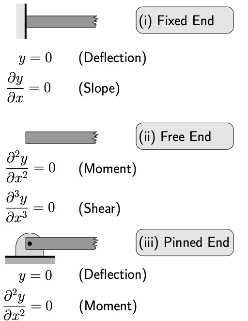
As can be seen there are four constants to be determined which requires that four boundary conditions be specified. These will often be determined with one pair of boundary conditions specified at each end, depending on the type of support. Figure 10.7 shows three of the most common support conditions and the pairs of boundary conditions that are associated with each type of support.
EXAMPLE
A uniform beam (density , cross–sectional area  , flexural rigidity ) of length is fixed at one end and free at the other.
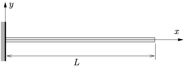
Determine expressions for the natural frequencies and associated mode shapes for this beam.
Complete Response of Lateral Motion of Beam
We have again found an infinite number of solutions which satisfy the equation of motion 10.26 given by
(10.33) ![\begin{equation*}y_n(x,t) = \ensuremath{\mathbb{Y}}_n(x) \biggl[ \hat{C}_n \, \sin{p_n t} +\hat{D}_n \, cos{p_n t} \biggr],\qquad n = 1,2, ... \infty\end{equation*}](https://engcourses-uofa.ca/wp-content/ql-cache/quicklatex.com-009b93e71a7e3d502afff71032b57f47_l3.png "Rendered by QuickLaTeX.com")
where  is the
  natural frequency and
  is the associated mode shape, both of which depend on the specific boundary conditions present. The general solution will then be a superposition of all of the solutions in 10.33,
(10.34) ![\begin{align*}y(x,t) =& \sum_{n=1}^{\infty} y_n(x,t) \nonumber \\y(x,t) =& \sum_{n=1}^{\infty}\ensuremath{\mathbb{Y}}_n(x) \biggl[ \hat{C}_n \, \sin{p_n t} + \hat{D}_n \, cos{p_n t} \biggr]\end{align*}](https://engcourses-uofa.ca/wp-content/ql-cache/quicklatex.com-d88f5f4ce3a2bc6d2b155969aa36e372_l3.png "Rendered by QuickLaTeX.com")
The constants  and
and  are to be determined from the initial conditions of the beam. If the initial displacement and velocity of the beam are specified as

then 10.34 gives

and can then be found from
(10.35) 
(10.36) 
where once again the orthogonality property of the mode shape has been used

This is once again beyond the scope of this course.