Engineering at Alberta Courses » Axial Vibrations of a Uniform Bar

Vibrations of Continuous Systems: Axial Vibrations of a Uniform Bar

Equation of Motion

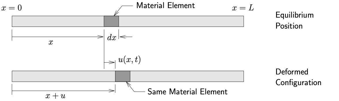
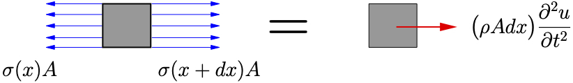
(a) Schematic of uniform bar undergoing longitudinal motion

(b) FBD/MAD of infinitesimal element
Figure 10.4: Axial vibrations of a uniform bar

Consider a uniform bar shown in Figure 10.4(a) which has a length $L$ , cross–sectional area $A$ and density $\rho$ (mass per unit volume). Let $u(x,t)$ measure the axial deformation of the material located at position $x$ in the equilibrium position. A FBD/MAD of an infinitesimal element of the beam is shown in Figure 10.4(b). Applying Newton’s Laws we get

$\stackrel{+}\rightarrow\sum F = ma:\qquad\sigma\bigl(x + dx\bigr) \cancel{A} - \sigma\bigl(x\bigr) \cancel{A} = \rho \cancel{A} dx \ensuremath{\frac{\partial^2 u}{\partial t^2}}$

For a linear elastic material

$\begin{equation*}\sigma = E\varepsilon\end{equation*}$

where $E$ is Young’s modulus and $\varepsilon$ is the axial strain given by

$\begin{equation*}\varepsilon = \frac{\partial u}{\partial x}\end{equation*}$

For small deformations we can make the approximation that

$\begin{equation*}\sigma\bigl(x\bigr) = E\Bigl(\frac{\partial u}{\partial x}\Bigr)\end{equation*}$

and

$\begin{equation*}\sigma\bigl(x + dx\bigr) = E\Bigl(\frac{\partial u}{\partial x} + \ensuremath{\frac{\partial^2 u}{\partial x^2}} dx \Bigr)\end{equation*}$

The equation of motion then becomes

$\begin{align*}E\Bigl({\frac{\partial u}{\partial x}} + \ensuremath{\frac{\partial^2 u}{\partial x^2}} dx \Bigr)- {E\Bigl(\frac{\partial u}{\partial x}\Bigr)} &= \rho dx \ensuremath{\frac{\partial^2 u}{\partial t^2}} \\[2mm]E \ensuremath{\frac{\partial^2 u}{\partial x^2}} {dx} &= \rho {dx} \, \ensuremath{\frac{\partial^2 u}{\partial t^2}}\end{align*}$

or finally

(10.19) $\begin{equation*}\boxed{\ensuremath{\frac{\partial^2 u}{\partial x^2}} = \dfrac{1}{\ensuremath{c}^2} \ensuremath{\frac{\partial^2 u}{\partial t^2}}}\end{equation*}$

where

(10.20) $\begin{equation*}\boxed{\ensuremath{c} = \sqrt{\dfrac{E}{\rho}}}\end{equation*}$

We recognize 10.19 once again as the wave equation. In this case $\ensuremath{c}$ is the speed of the axial waves traveling along the beam as opposed to the transverse motions for the cable seen previously.

Solution for the Axial Response of the Beam

Following our previous solution procedure for cables, we assume a solution of the form

$\begin{equation*}u(x,t) = \ensuremath{\mathbb{U}}(x)\,\ensuremath{\mathbb{T}}(t)\end{equation*}$

Upon substitution into the equation of motion and proceeding as before we find that

(10.21a) $\begin{equation*}\ensuremath{\mathbb{U}}(x) = \hat{A} \sin\biggl(\frac{p x}{\ensuremath{c}}\biggr) + \hat{B} \cos\biggl(\frac{p x}{\ensuremath{c}}\biggr)\end{equation*}$

(10.21b) $\begin{equation*}\ensuremath{\mathbb{T}}(t) = \hat{C} \sin(p t}) + \hat{D} \cos(p t)\end{equation*}$

As a result the total solution for the axial motions becomes

(10.22) $\begin{equation*}u(x,t) = \underbrace{\biggl[ \hat{A} \sin\biggl(\frac{p x}{\ensuremath{c}}\biggr) + \hat{B} \cos\biggl(\frac{p x}{\ensuremath{c}}\biggr) \biggr]}_{\text{Mode shape (function of $x$)}}\underbrace{\biggl[ \hat{C} \sin(p t) + \hat{D} \cos(p t) \biggr]}_{\text{Harmonic motion (function of $t$)}}\end{equation*}$

Once again the constants $\hat{A}$ and $\hat{B}$ are determined from the boundary conditions while $\hat{C}$ and $\hat{D}$ are subsequently determined from the initial conditions.

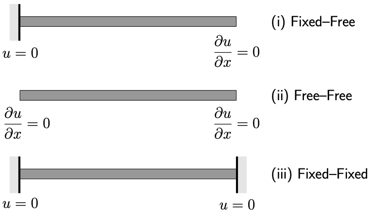
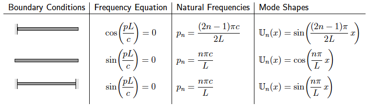
Some common boundary conditions for axial motions of beams are illustrated in Figure 10.5. The results for some common beam configurations are shown in Table 10.2. The procedure to find these results is the same as was followed for the vibrating cable considered earlier.

Open Educational Resources

Vibrations of Continuous Systems: Axial Vibrations of a Uniform Bar

Equation of Motion

Solution for the Axial Response of the Beam

Leave a Reply Cancel reply