Engineering at Alberta Courses » Response of Spring

Transient Vibrations: Response of Spring–Mass System to a Step Function

As we have discussed so far, in many situations the long term (steady state) response of a vibrating system is of interest. For example, for a motor that will operate more than 99% of the time at a fixed operating speed we would typically want to investigate the response at that speed so an appropriate vibration isolation system could be designed.

On the other hand, there are times when it is the transient response of the system that is of interest.

For the motor example above, we may be concerned about the response at startup, particularly if the system passes through resonance.
The response of an automobile suspension system when a pothole or other obstacle in the road is encountered.
The response of various mechanical systems to shock loading.

In these situations, the loading isn’t periodic or is applied for a short period of time. We will look at the responses for some specific examples. We will limit ourselves generally to undamped systems for simplicity so that the general form of the equation of motion we are concerned with here is

(7.1) $m \ddot{x} + k x = F(t)$

where $F(t)$ is the disturbing force under consideration.

Response of a Spring-Mass System to a Step Function

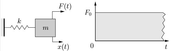
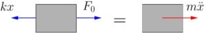
Consider a simple spring–mass system subjected to a rectangular step load as shown in Figure 7.1(a). We would like to find the response of the mass to this transient loading condition. Figure 7.1(b) shows the associated FBD/MAD. The equation of motion obtained using Newton’s laws is

$\begin{equation*}\stackrel{+}{\rightarrow}\sum F = ma:\qquad -k x + F_0 = m \ddot{x}\end{equation*}$

(7.2) $\begin{equation*}\label{eq:StepFunctionEOM}m \ddot{x} + kx = F_0, \qquad\qquad t>0\end{equation*}$

As usual, the solution is composed of the homogeneous and particular solutions

$\begin{equation*}x(t) = A \sin{pt} + B \cos{pt} + x_P(t)\end{equation*}$

For the RHS in (7.2), the particular solution is

$\begin{equation*}x_P(t) = \frac{F_0}{k}\end{equation*}$

so the total solution becomes

$\begin{equation*}x(t) = A \sin{pt} + B \cos{pt} + \frac{F_0}{k}\end{equation*}$

If we start with the initial conditions

$\begin{equation*}x(0) = 0, \qquad \dot{x}(0) = 0,\end{equation*}$

the constants* become

$\begin{equation*}A = 0,\qquad B = -\frac{F_0}{k},\end{equation*}$

so that the total solution is

(7.3) $\begin{equation*}\label{eq:StepFunctionSolution}\boxed{x(t) = \frac{F_0}{k} \Bigl[ 1 - \cos{pt} \Bigr]}\end{equation*}$

*Note that the total solution (including the particular solution) must be used to determine the arbitrary constants which arise from the homogeneous solution.

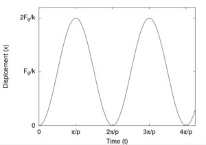
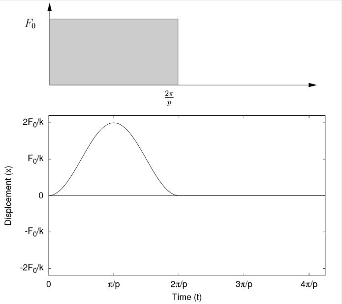
Figure 7.2: Response of simple spring–mass system to applied step load

This response is illustrated in Figure 7.2. We can see that the maximum displacement of the mass is $2\frac{F_0}{k}$ which is twice the deflection that would have resulted if the load were applied statically. Now consider what happens if the step load is “turned off” at some time $\hat{t}$ . After this time, since there is no longer any applied force, the system undergoes free vibrations given by

$\begin{equation*}x(t) = \hat{A} \sin{pt} + \hat{B} \cos{pt}, \qquad\qquad t>\hat{t}\end{equation*}$

where $\hat{A}$ and $\hat{B}$ need to be evaluated at the “initial” conditions ( $t=\hat{t}\,$ ) which depend on the time $\hat{t}$ at which the force was removed. The response of the mass while the step load is applied is given in equation (7.3). Similarly, the velocity of the mass during this period is, by differentiation,

$\begin{equation*}\dot{x}(t) = \frac{F_0 p}{k} \sin{pt}\end{equation*}$

Therefore, at the time $\hat{t}$ when the load is removed, the “initial” conditions are

$\begin{equation*}x(\hat{t}) = \frac{F_0}{k} \Bigl[ 1 - \cos{p\hat{t}} \Bigr], \qquad\dot{x}(\hat{t}) = \frac{F_0}{k}{\sin{p\hat{t}}}\end{equation*}$

which can be used to find $\hat{A}$ and $\hat{B}$ .

Consider two specific examples

(1) ${\hat{t} = \dfrac{2 \pi}{p}}$

$\begin{alignat*}{2}x(\hat{t}) &= \frac{F_0}{k} \Bigl[ 1 - \cos{2 \pi} \Bigr] & &= 0 \\[2mm]\dot{x}(\hat{t}) &= \frac{F_0 p}{k} \sin{2 \pi} & & =0\end{alignat*}$

As a result,

$\begin{equation*}\hat{A} = 0, \qquad \hat{B} = 0\end{equation*}$

so the response in this case is

$\begin{equation*}x(t) = \begin{cases}\dfrac{F_0}{k\rule[-3mm]{0pt}{0pt}} \Bigl[ 1 - \cos{pt}], & t \le \dfrac{2 \pi}{p}\\0, \qquad\qquad\qquad & t > \dfrac{2 \pi}{p} \\\end{cases}\end{equation*}$

(2) ${\hat{t} = \dfrac{\pi}{p}}$

$\begin{alignat*}{2}x(\hat{t}) &= \frac{F_0}{k} \Bigl[ 1 - \cos{\pi} \Bigr] & &= 2 \frac{F_0}{k} \\[2mm]\dot{x}(\hat{t}) &= \frac{F_0 p}{k} \sin{\pi} & &=0\end{alignat*}$

As a result,

$\begin{equation*}\hat{A} = 0, \qquad \hat{B} = \frac{2 F_0}{k}\end{equation*}$

so the response in this case is

$\begin{equation*}x(t) = \begin{cases}\dfrac{F_0}{k\rule[-5mm]{0pt}{0pt}} \Bigl[ 1 - \cos{pt} \Bigr], & t \le \dfrac{\pi}{p}\\-\dfrac{2 F_0}{k} \cos{pt}, \qquad\qquad & t > \dfrac{\pi}{p} \\\end{cases}\end{equation*}$

These responses are shown in Figure 7.3. As these responses clearly show, the transient nature of the applied loading can have a significant effect on the resulting response.

Figure 7.3: Response of simple spring–mass system to applied step load which is subsequently removed
(a) τ =2π/p

Figure 7.3: Response of simple spring–mass system to applied step load which is subsequently removed
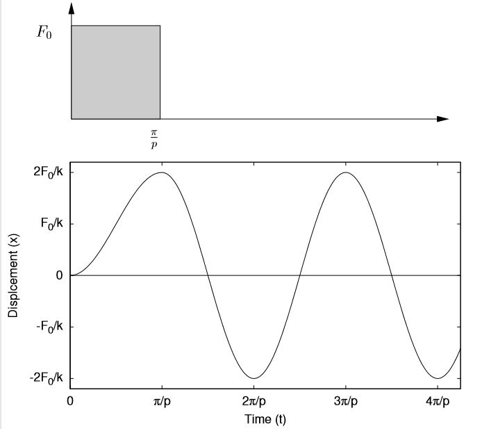
(b) τ = π/p

The previous responses can be understood on a physical basis. In the first case, $F_0$ is applied to a system originally in its equilibrium position. When $F_0$ is applied, the effect is to shift the new equilibrium position a distance $\frac{F_0}{k}$ as shown in Figure 7.4.

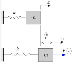
This image has an empty alt attribute; its file name is EquilibriumPosSchematic-300x256.jpg — Figure 7.4: Shift of equilibrium position

At time $t=0$ (immediately after the application of $F_0$ ), the mass is apparently in a position (top of Figure 7.4) where it is displaced from its new equilibrium position. If we measure the displacement of the mass from the new equilibrium position as $y$ and neglect both the applied force $F_0$ and the new equilibrium stretch in the spring (as we did regularly when gravity was present), we then have a free vibration problem with the initial conditions

$\begin{equation*}y(0) = -\frac{F_0}{k},\qquad \dot{y} = 0,\end{equation*}$

so the free vibration response is

$\begin{equation*}y(t) = -\frac{F_0}{k} \cos{pt}.\end{equation*}$

However, since $x = y + \frac{F_0}{k}$ , we can write the response in terms of $x$ as

$\begin{equation*}x(t) = \frac{F_0}{k} \Bigl[ 1 - \cos{pt} \Bigr]\end{equation*}$

as before.

The two cases shown in Figure 7.3 can be understood on similar principles. When the force $F_0$ is removed, the equilibrium position of the system returns to its original position. The time at which the force $F_0$ is removed determines the initial conditions for the subsequent free vibration problem, which leads to the responses shown.

Response of Spring–Mass System to an Impulse

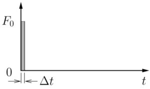
Figure 7.5: Impulse Loading

We now consider the response of a spring–mass system subjected to an impulsive loading shown in Figure 7.5. (Note that the quantity $F_0 \Delta t$ is the area under the force-time curve and is known as the impulse applied to the system.) Here the time $\hat{t}$ at which the load is removed is small ( $\Delta t$ ) so that

$\begin{equation*}p\hat{t} = p \Delta t \ll 1\end{equation*}$

In such a case,

$\begin{equation*}\cos{p\hat{t}} \approx 1\\[1mm]\end{equation*}$

$\begin{equation*}\sin{p\hat{t}} \approx p\hat{t} = p\,\Delta t\end{equation*}$

The “initial” conditions are approximately

$x(\hat{t}) \approx \frac{F_0}{k}\left(1-\cancelto{1}{\cos pt}\right) = 0$

$\dot{x}(\hat{t}) \approx \frac{F_0 p}{k}p\Delta t = F_0 \cancelto{\frac{1}{m}}{\frac{p^2}{k}}\Delta t = \frac{F_0 \Delta t}{m}$

so the initial conditions (after impulse has been applied) become

$\begin{equation*}x(0) \approx x(\hat{t}) = 0\end{equation*}$

$\begin{equation*}\\[1mm]\dot{x}(0) \approx \dot{x}(\hat{t}) = \frac{F_0 \Delta t}{m}\end{equation*}$

The constants $\hat{A}$ and $\hat{B}$ are then

$\begin{equation*}\hat{A} = \frac{F_0 \Delta t}{m p}, \qquad \hat{B} = 0\end{equation*}$

so the response becomes

(7.4) $\begin{equation*}\label{eq:ImpulseResponse}\boxed{x(t) = \frac{F_0 \Delta t}{m p} \sin{pt}, \qquad t>0}\end{equation*}$

This response will play an important role later when we consider the method of convolution.

Aside

We can obtain this result another way by applying the basic principle of impulse and momentum for our system.

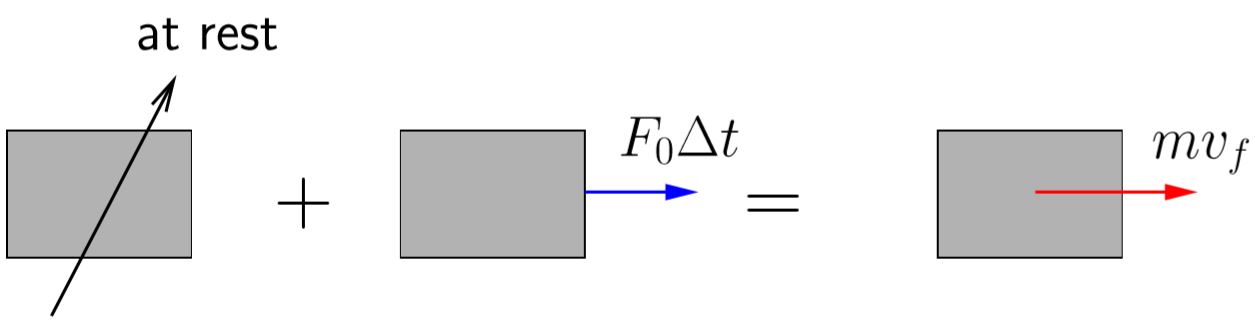
Figure 7.6: Impulse–momentum diagram for mass m

Figure 7.6 shows an impulse–momentum diagram for our simple spring mass system when the impulsive load is applied. The system is initially at rest and after the impulse has been applied has a resulting velocity $v_f$ . (Note that the force of the spring is not included in the diagram. The assumption is that the impulse is applied fast enough that the mass does not have time to move while the impulse is being applied. Since the mass does not move, the force in the spring remains unchanged. We say that the force of the spring is non-impulsive.)