Non-Harmonic Periodic Forcing Functions: Fourier Analysis
To this point we have only considered harmonic forcing functions (e.g. sine). These are examples of periodic functions since they repeat themselves after a specific period of time. However, harmonic functions are not the only type of periodic function. There are many others, some typical examples of which are shown in Figure 6.1
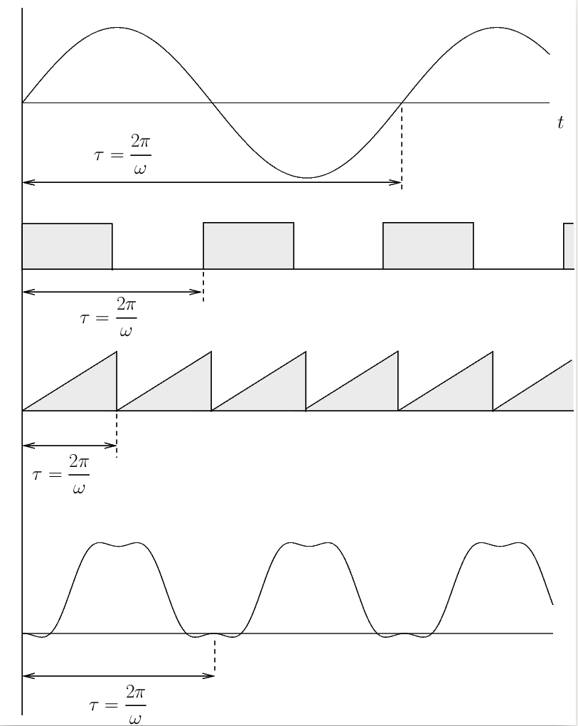
It would be useful to be able to determine the response of a single degree of freedom system to these other periodic forcing functions as well. Fortunately much of what we have already studied can be applied.
Fourier Analysis
Whenever we have a periodic forcing function  with period
  it can always be expressed as a Fourier series (a sum of harmonic functions) as
(6.1) ![\[F(t) = \frac{a_0}{2} + \sum_{j=1}^\infty a_j \ensuremath{\cos\left(j \omega t\right)} + \sum_{j=1}^\infty b_j \ensuremath{\sin\left(j \omega t\right)},\]](https://engcourses-uofa.ca/wp-content/ql-cache/quicklatex.com-cb2d5bc525bbb2117b3ef802f9eda69f_l3.png "Rendered by QuickLaTeX.com")
where
(6.2a) ![\[a_0 = \frac{2}{\tau} \int_0^{\tau} F(t) dt,\qquad (= 2 F_{\mathrm{AVE}}),\]](https://engcourses-uofa.ca/wp-content/ql-cache/quicklatex.com-7fd2840d35b07653a1276e9962fd9d40_l3.png "Rendered by QuickLaTeX.com")
(6.2b) ![\[a_j = \frac{2}{\tau} \int_0^{\tau} F(t) \ensuremath{\cos\left(j \omega t\right)} dt, \qquad j=1,2,\dots,\infty,\]](https://engcourses-uofa.ca/wp-content/ql-cache/quicklatex.com-53c8b5145aab143b81f1d0342e10b909_l3.png "Rendered by QuickLaTeX.com")
(6.2c) ![\[b_j = \frac{2}{\tau} \int_0^{\tau} F(t) \ensuremath{\sin\left(j \omega t\right)} dt, \qquad j=1,2,\dots,\infty.\]](https://engcourses-uofa.ca/wp-content/ql-cache/quicklatex.com-62f6ccb80f21db9e73b76baa94055cc0_l3.png "Rendered by QuickLaTeX.com")
For a given periodic function
, the coefficients  ,
,  and
and  (
( ) can be uniquely determined.
With this expansion of the forcing function, the equation of motion for the damped spring-mass system
![\[m \ddot{x} + c \dot{x} + k x = F(t)\]](https://engcourses-uofa.ca/wp-content/ql-cache/quicklatex.com-27c9f5a4060e1b45e8a3e4ff674a88c5_l3.png "Rendered by QuickLaTeX.com")
becomes
(6.3) ![\[m \ddot{x} + c \dot{x} + k x = \frac{a_0}{2} + \sum_{j=1}^\infty a_j \ensuremath{\cos\left(j \omega t\right)} + \sum_{j=1}^\infty b_j \ensuremath{\sin\left(j \omega t\right)}\]](https://engcourses-uofa.ca/wp-content/ql-cache/quicklatex.com-4c55a8724d2eec7f2042559d29277e20_l3.png "Rendered by QuickLaTeX.com")
To find the steady state solution to (6.3) we make use of the principle of superposition to express the total solution as the sum of the individual solutions to each term on the right hand side. That is, the solution is the sum of the solutions to
(6.4a) ![\[m \ddot{x} + c \dot{x} + k x = \frac{a_0}{2}\]](https://engcourses-uofa.ca/wp-content/ql-cache/quicklatex.com-b7a291d02f07ce343b6eaac3a5400f9e_l3.png "Rendered by QuickLaTeX.com")
(6.4b) ![\[m \ddot{x} + c \dot{x} + k x = a_j \ensuremath{\cos\left(j \omega t\right)}, \qquad j=1,2,\dots,\infty\]](https://engcourses-uofa.ca/wp-content/ql-cache/quicklatex.com-329117ee6209192bdea9d585159c7721_l3.png "Rendered by QuickLaTeX.com")
(6.4c) ![\[m \ddot{x} + c \dot{x} + k x = b_j \ensuremath{\sin\left(j \omega t\right)}, \qquad j=1,2,\dots,\infty\]](https://engcourses-uofa.ca/wp-content/ql-cache/quicklatex.com-6f51edb0a7eeb58d190a28e7c3578e81_l3.png "Rendered by QuickLaTeX.com")
The steady state solution to (6.4a) is simply
(6.5) ![\[x(t) = \frac{a_0}{2k}\]](https://engcourses-uofa.ca/wp-content/ql-cache/quicklatex.com-fa224fea4c56056716e655103b99c28b_l3.png "Rendered by QuickLaTeX.com")
Aside
We have previously shown that the steady state solution to
![\[m \ddot{x} + c \dot{x} + k x = F_0 \sin \omega t\]](https://engcourses-uofa.ca/wp-content/ql-cache/quicklatex.com-de5661c3530d0084d406a3a0fa164a47_l3.png "Rendered by QuickLaTeX.com")
is
![\[x(t) = \frac{\dfrac{F_0}{k}}{\ensuremath{\sqrt{\Bigl[1-\ensuremath{\bigl(\frac{\omega}{\ensuremath{p}}\bigr)}^2\Bigr]^2 + \Bigl[2 \zeta \ensuremath{\frac{\omega}{\ensuremath{p}}} \Bigr]^2}}} \sin (\omega t - \phi), \qquad \phi = \tan^{-1} \Biggl[ \frac{2 \zeta \ensuremath{\frac{\omega}{\ensuremath{p}}}}{1-\ensuremath({\frac{\omega}{\ensuremath{p}}})^2} \Biggr].\]](https://engcourses-uofa.ca/wp-content/ql-cache/quicklatex.com-0bdcb8042870554bc9732bbc1c20c051_l3.png "Rendered by QuickLaTeX.com")
Following the same procedure, it is straightforward to show that the solution to
![\[m \ddot{x} + c \dot{x} + k x = F_0 \cos \omega t\]](https://engcourses-uofa.ca/wp-content/ql-cache/quicklatex.com-c27bb75ee7c4953f8f5c693c464d4c93_l3.png "Rendered by QuickLaTeX.com")
is similarly
![\[x_P(t) = \frac{\dfrac{F_0}{k}}{\ensuremath{\sqrt{\Bigl[1-\ensuremath{\bigl(\frac{\omega}{\ensuremath{p}}\bigr)}^2\Bigr]^2 + \Bigl[2 \zeta \ensuremath{\frac{\omega}{\ensuremath{p}}} \Bigr]^2}}} \cos (\omega t - \phi), \qquad\phi = \tan^{-1} \Biggl[ \frac{2 \zeta \ensuremath{\frac{\omega}{\ensuremath{p}}}}{1-\ensuremath({\frac{\omega}{\ensuremath{p}}})^2} \Biggr]\]](https://engcourses-uofa.ca/wp-content/ql-cache/quicklatex.com-282af149f4e64a3e33741ef0c0630727_l3.png "Rendered by QuickLaTeX.com")
The steady state solution to equations (6.4b) and (6.4c) are
(6.6) ![\[\newcommand{\COS}[1]{\ensuremath{\cos\bigl({#1}\bigr)}}x(t) = \frac{\dfrac{a_j}{k}}{\sqrt{\Bigl[ 1-\Bigl(\frac{j \omega}{\ensuremath{p}} \Bigr)^2 \Bigr]^2 + \Bigl[ 2 \zeta \frac{j \omega}{\ensuremath{p}} \Bigr]^2} }\COS{j \omega t - \phi_j}\]](https://engcourses-uofa.ca/wp-content/ql-cache/quicklatex.com-7e169f84621e116ce399ca68321da57b_l3.png "Rendered by QuickLaTeX.com")
and
(6.7) ![\[\newcommand{\SIN}[1]{\ensuremath{\sin\bigl({#1}\bigr)}}x(t) = \frac{\dfrac{b_j}{k}}{\sqrt{\Bigl[ 1-\Bigl(\frac{j \omega}{\ensuremath{p}} \Bigr)^2 \Bigr]^2 + \Bigl[ 2 \zeta \frac{j \omega}{\ensuremath{p}} \Bigr]^2}}\SIN{j \omega t - \phi_j}\]](https://engcourses-uofa.ca/wp-content/ql-cache/quicklatex.com-9a470b95fd0fbb9fa1a2e636979d7ebe_l3.png "Rendered by QuickLaTeX.com")
respectively where
(6.8) ![\[\phi_j = \tan^{-1} \Biggl[ \frac{2 \zeta \frac{j \omega}{\ensuremath{p}}}{1-\bigl(\frac{j \omega}{\ensuremath{p}} \bigr)^2} \Biggr]\]](https://engcourses-uofa.ca/wp-content/ql-cache/quicklatex.com-ab0ef90095bcfa9b0e83dd24df154389_l3.png "Rendered by QuickLaTeX.com")
Therefore the steady state solution to equation (6.3) is given by
(6.9) ![\[\newcommand{\SIN}[1]{\ensuremath{\sin\bigl({#1}\bigr)}}\newcommand{\COS}[1]{\ensuremath{\cos\bigl({#1}\bigr)}}\begin{split}x(t) = \frac{a_0}{2k} + \sum_{j=1}^{\infty} \frac{\dfrac{a_j}{k}}{\sqrt{\Bigl[ 1-\Bigl(\frac{j \omega}{\ensuremath{p}} \Bigr)^2 \Bigr]^2 + \Bigl[ 2 \zeta \frac{j \omega}{\ensuremath{p}} \Bigr]^2}}\COS{j \omega t - \phi_j} \\+ \sum_{j=1}^{\infty} \frac{\dfrac{b_j}{k}}{\sqrt{\Bigl[ 1-\Bigl(\frac{j \omega}{\ensuremath{p}} \Bigr)^2 \Bigr]^2 + \Bigl[ 2 \zeta \frac{j \omega}{\ensuremath{p}} \Bigr]^2}}\SIN{j \omega t - \phi_j}\end{split}\]](https://engcourses-uofa.ca/wp-content/ql-cache/quicklatex.com-288b82370dea15f03eaa781cce7ae4ad_l3.png "Rendered by QuickLaTeX.com")
where
 is given by (6.8)
Note:
- The amplitude and phase angle for the
 frequency depend on
  and are not constants
 - The terms with frequency component
 closest to
  will have the largest dynamic magnification factor.
 - As continues to increase, the amplitude of the terms decreases (due to the dynamic magnification factor). As a result, in practice a reasonably accurate solution can be obtained using only the first few terms in the expansion in equation (6.3).
- If the periodic forcing function is sufficiently complex or is determined experimentally the integrations in equations (6.2b) and (6.2c) may not be available analytically. In these case the Fourier coefficients can be approximated numerically.
We can consider the period to be broken into
  (an even number) of equally spaced time intervals
  so that
  .
.
If represent the values of at the times
  then the Fourier coefficients can be approximated as
Once these coefficients are known, we can proceed as before with replaced by
  .
. - The solutions shown are for the steady state only. If we are interested in the transient solution as well, we must add the solution to
(6.10)
to our solution. The solution to (6.10) for the underdamped case is
in which the two constants![\begin{alignat*}{2} x(t) = e^{-\zeta p t} \Bigl[ A \sin(\sqrt{1-\zeta^2}pt) + B \cos(\sqrt{1-\zeta^2}pt)\Bigr] \end{alignat*}](https://engcourses-uofa.ca/wp-content/ql-cache/quicklatex.com-d971a4bdb5880bd174a6260f3e77902f_l3.png "Rendered by QuickLaTeX.com")
 and
and  are determined using initial conditions. These constants must be determined using the complete solution, so the Fourier coefficients need to be determined before and can be evaluated.
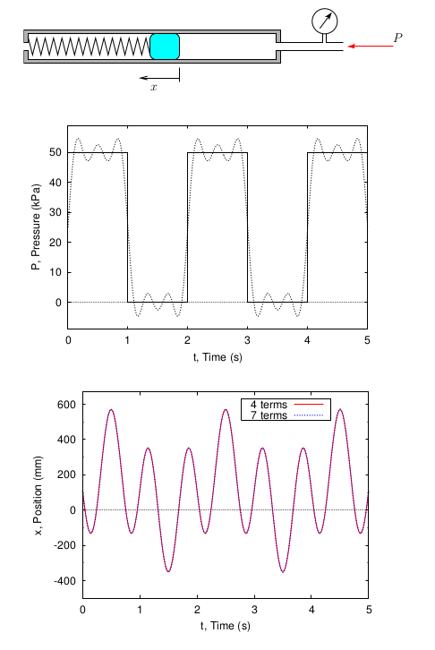
EXAMPLE
A 3.68 kg slider is placed in a smooth tube with an internal diameter of 40 mm. The spring has a stiffness of 284 N/m. One side of the tube is open to the atmosphere. The pressure on the other side varies periodically as shown in the graph.
Determine the steady state response of the slider