
Forced Vibrations of Damped Single Degree of Freedom Systems: Base Excitation in a Damped System
We can also consider the response of a damped spring–mass system subjected to base excitation. Among other applications, these results are useful when considering the operation of transducers that measure vibrations.
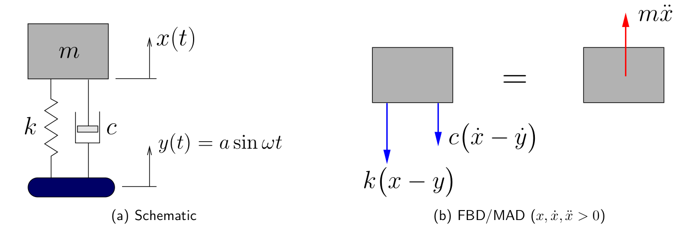
Figure 5.11(a) illustrates such a situation schematically while Figure 5.11(b) shows the corresponding FBD/MAD diagram. Applying Newton’s Laws we find
(5.23) 
(5.24) ![\[m \ddot{x} + c\dot{x} +k x = k a \sin \omega t + c a \omega \cos \omega t\]](https://engcourses-uofa.ca/wp-content/ql-cache/quicklatex.com-fcf83d747581b22fa4cb90a6b5745445_l3.png "Rendered by QuickLaTeX.com")
This can also be expressed as
![\[m \ddot{x} + c\dot{x} +kx = \ensuremath{\mathbb{R}} \sin{(\omega t - \alpha)}\]](https://engcourses-uofa.ca/wp-content/ql-cache/quicklatex.com-c38d43fee8c8a9a11bbe8325756a824c_l3.png "Rendered by QuickLaTeX.com")
where
![\[\ensuremath{\mathbb{R}} = a \sqrt{k^2 + \bigl(c \omega\bigr)^2}, \qquad\alpha = \tan^{-1}{\biggl[\frac{-c \omega}{k}\biggr]}\]](https://engcourses-uofa.ca/wp-content/ql-cache/quicklatex.com-65bbdb8ef08bdcb0db37ac3f4e8b4e1b_l3.png "Rendered by QuickLaTeX.com")
As a result, we can see that the base excitation is equivalent to applying a harmonic force of magnitude  to a mass with a fixed base. We have previously found the steady state solution for such a case (equations (5.7) and (5.9)) which here becomes
![\[x(t) = \frac{a \sqrt{k^2 + \bigl(c \omega\bigr)^2}}{\ensuremath{\sqrt{(k-m\omega)^2 + (c\omega)^2}}}\sin{(\omega t - \alpha -\phi_1)}\]](https://engcourses-uofa.ca/wp-content/ql-cache/quicklatex.com-dc1419baf6930ac888860ae403898004_l3.png "Rendered by QuickLaTeX.com")
where
![\[\phi_1 = \tan^{-1}{\Biggl[\frac{c \omega}{k-m\omega^2}\Biggr]}\]](https://engcourses-uofa.ca/wp-content/ql-cache/quicklatex.com-862bdd2e3e7255055acb9b1391e21bf3_l3.png "Rendered by QuickLaTeX.com")
Therefore we could write the response as
![\[x(t) = \mathbb{X} \sin{(\omega t - \Phi)}\]](https://engcourses-uofa.ca/wp-content/ql-cache/quicklatex.com-763150f42475c9f70fb1178c09c37574_l3.png "Rendered by QuickLaTeX.com")
where
![\[\frac{\mathbb{X}}{a} = \frac{\sqrt{k^2 + \bigl(c \omega\bigr)^2}}{\ensuremath{\sqrt{(k-m\omega)^2 + (c\omega)^2}}}\]](https://engcourses-uofa.ca/wp-content/ql-cache/quicklatex.com-f5fbd97f5ade96adbfb3ae4051ef19f0_l3.png "Rendered by QuickLaTeX.com")
and
![\[\Phi = \alpha + \phi_1 =\tan^{-1}{\biggl[\frac{-c \omega}{k}\biggr]} +\tan^{-1}{\biggl[\frac{c \omega}{k-m\omega^2}\biggr]}\]](https://engcourses-uofa.ca/wp-content/ql-cache/quicklatex.com-5f0b152a78b6bdb32708bbd7f9602cc1_l3.png "Rendered by QuickLaTeX.com")
However, this in often not the most convenient form for the phase angle. It can be shown (after some algebra) that
![\[\tan \Phi = \frac{m c \omega^3}{k\bigl(k-m\omega^2\bigr)+\bigl(c \omega\bigr)^2 }\]](https://engcourses-uofa.ca/wp-content/ql-cache/quicklatex.com-d25cf5dd909837d8d5c6fe6568b6d15d_l3.png "Rendered by QuickLaTeX.com")
which can also be expressed in non-dimensional form as
![\[\tan \Phi = \frac{2 \zeta \left(\ensuremath{\frac{\omega}{\ensuremath{p}}}\right)^3}{1 + \bigl(4\zeta^2-1\bigr)\left(\ensuremath{\frac{\omega}{\ensuremath{p}}}\right)^2}\]](https://engcourses-uofa.ca/wp-content/ql-cache/quicklatex.com-b1b1a2569f3708bed52627a91d65e557_l3.png "Rendered by QuickLaTeX.com")
To summarize, the response of the damped spring–mass system to harmonic base excitation is given by
(5.25) ![\[x(t) = \mathbb{X} \sin{(\omega t - \Phi)}\]](https://engcourses-uofa.ca/wp-content/ql-cache/quicklatex.com-ac1ad48803ebb9382e12d37ae57c8b82_l3.png "Rendered by QuickLaTeX.com")
where
(5.26) ![\[\frac{\mathbb{X}}{a} = \frac{\sqrt{k^2 + \bigl(c \omega\bigr)^2}}{\ensuremath{\sqrt{(k-m\omega)^2 + (c\omega)^2}}}\]](https://engcourses-uofa.ca/wp-content/ql-cache/quicklatex.com-b9bacd150cc4dd1e7d4d3de9a636c25f_l3.png "Rendered by QuickLaTeX.com")
and
(5.27) ![\[\Phi = \tan^{-1} \Biggl[\frac{m c \omega^3}{k\bigl(k-m\omega^2\bigr)+\bigl(c \omega\bigr)^2 } \Biggr]\]](https://engcourses-uofa.ca/wp-content/ql-cache/quicklatex.com-79fcb529c5389771b3b4cf64a550d72e_l3.png "Rendered by QuickLaTeX.com")
In dimensionless form these become
(5.28) ![\[\boxed{ \frac{\mathbb{X}}{a} = \frac{\sqrt{1 + \bigl(2 \zeta \ensuremath{\frac{\omega}{\ensuremath{p}}} \bigr)^2}}{\ensuremath{\sqrt{\left[1-\left(\ensuremath{\frac{\omega}{\ensuremath{p}}}\right)^2\right]^2 + \left[2 \zeta \ensuremath{\frac{\omega}{\ensuremath{p}}} \right]^2}}}}\]](https://engcourses-uofa.ca/wp-content/ql-cache/quicklatex.com-8f7edeae698cff76b94a81a9c981621d_l3.png "Rendered by QuickLaTeX.com")
and
(5.29) ![\[\boxed{ \Phi = \tan^{-1} \Biggl[\frac{2 \zeta \left(\ensuremath{\frac{\omega}{\ensuremath{p}}}\right)^3}{1 + \bigl(4\zeta^2-1\bigr)\left(\ensuremath{\frac{\omega}{\ensuremath{p}}}\right)^2}\Biggr]}\]](https://engcourses-uofa.ca/wp-content/ql-cache/quicklatex.com-731958d02e04d2333ce7dc794ff4390a_l3.png "Rendered by QuickLaTeX.com")
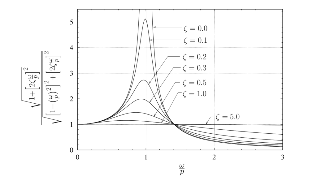
The term  can be thought of as the dynamic magnification factor in this situation as it represents the ratio of the amplitude of the motion of the mass to the amplitude of motion of the base.
Figure 5.12 illustrates this relationship. We can see that this factor is exactly the same as the transmissibility for the forced damped situation considered previously (equation (5.19) and Figure 5.7). Therefore the problem of isolating a mass from the motion of the base is essentially the same problem as preventing a disturbing force acting on the mass from being transmitted to the supporting structure (the base).
EXAMPLE
An instrument package of mass  is to be isolated from a vibrating surface which is moving with an amplitude
  at a frequency of 600 RPM.
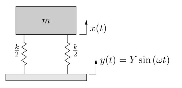
(a) What should the natural frequency of the system be if the maximum amplitude of the instrument package is to be  of ?
of ?
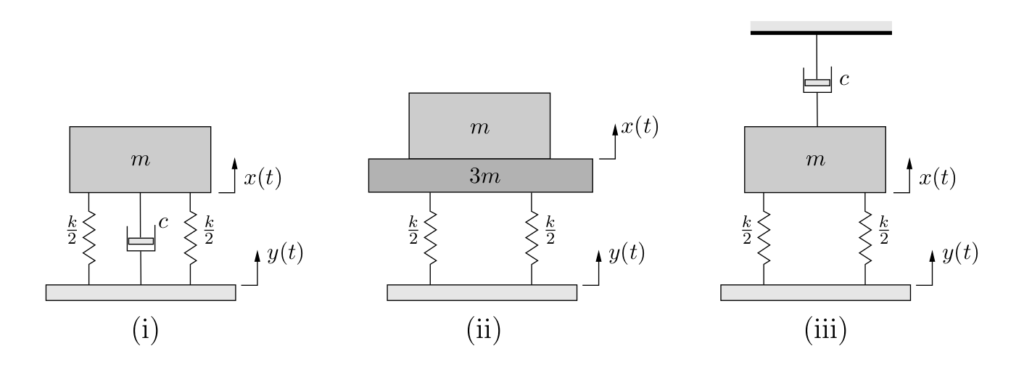
(b) In order to reduce the amplitude of oscillation even further, several ideas (illustrated below) are proposed to improve the situation. Evaluate each of these ideas and determine if it will improve or worsen the situation. Use a combination of calculations and diagrams to support your reasoning.
(i) A damper is added between the mass and vibrating surface which provides a damping ratio of 
(ii) An inertia mass equal to  is added on the same supports.
(iii) A damper is added between the instrument package and a fixed support to provide a damping ratio of . (Note: start from the differential equation of motion.)
EXAMPLE
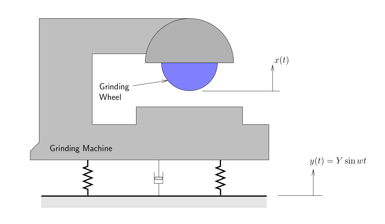
A precision grinding machine is supported on an isolator that has a stiffness of 1 MN/m and a viscous damping constant of 1 kN·s/m. The floor on which the machine is mounted is subjected to a harmonic disturbing force due to the operation of a unbalanced engine in the vicinity of the grinding machine operating at a speed of 6000 RPM. Determine the maximum acceptable amplitude of the floor motion () if the resulting amplitude of vibration of the grinding wheel is restricted to be  m. Assume that the grinding machine and the wheel are a rigid body of weight 5000 N.
Relative Motion Between the Mass and the Base
In the previous section we considered the response of a damped spring–mass system subjected to harmonic base excitation and found the absolute response of the mass. Those results are not always the most convenient to use. For example, in many vibration measurement instruments we usually directly measure only the relative motion between the mass and the base and then try to use this measurement to infer the underlying motion of the base (which is typically what we would be trying to measure).
Considering Figure 5.11(a) once again, the relative motion  between the mass and the base
is given by
![\[z(t) = x(t)-y(t).\]](https://engcourses-uofa.ca/wp-content/ql-cache/quicklatex.com-3bc936c8977fe2caacf0ad30395e78c2_l3.png "Rendered by QuickLaTeX.com")
However, as we have seen previously there is a phase difference  between
  and
and  , given by equation (5.29), which must be taken into account. For example we could take our previous solutions and expand them using trigonometric identities to account for this phase difference. An alternative (and often easier) approach is to consider the relative motion directly.
Since
![\[z = x - y\]](https://engcourses-uofa.ca/wp-content/ql-cache/quicklatex.com-ffa13ad9130af85dfc43250ae061e45f_l3.png "Rendered by QuickLaTeX.com")
we can write

The original equation of motion in (5.23)
![\[m \ddot{x} + c\bigl(\dot{x}-\dot{y}\bigr) + k\bigl(x-y\bigr) = 0\]](https://engcourses-uofa.ca/wp-content/ql-cache/quicklatex.com-d4478d1685abcc99e950e8c7f54bd50a_l3.png "Rendered by QuickLaTeX.com")
can then be written as
![\begin{align*} m \Bigl[ \ddot{z} + \ddot{y} \Bigr] + c \dot{z} + k z &= 0, \\ m \ddot{z} + c \dot{z} + k z &= -m \ddot{y}. \end{align*}](https://engcourses-uofa.ca/wp-content/ql-cache/quicklatex.com-d061f24e7c1c52f1cabd8d173d765839_l3.png "Rendered by QuickLaTeX.com")
However, since  ,
,  so the equation of motion becomes
(5.30) ![\[m \ddot{z} + c \dot{z} + k z = \underbrace{m a \omega^2\rule[-1mm]{0pt}{0pt}}_{\text F_0} \sin \omega t\]](https://engcourses-uofa.ca/wp-content/ql-cache/quicklatex.com-af037b7280123e991663855725e984d8_l3.png "Rendered by QuickLaTeX.com")
We note that this equation is identical to that obtained for the forced vibration situation (and particularly the case of a rotating imbalance) which we have already considered. The solution to this equation is therefore
(5.31) ![\[z(t) = \mathbb{Z} \sin (\omega t - \phi)\]](https://engcourses-uofa.ca/wp-content/ql-cache/quicklatex.com-a5b7b0d9317f4ae817a1de9132dce2e1_l3.png "Rendered by QuickLaTeX.com")
where
(5.32) ![\[\mathbb{Z} = \frac{\dfrac{m a \omega^2}{k}}{\ensuremath{\sqrt{\Bigl[1-\ensuremath{\bigl(\frac{\omega}{\ensuremath{p}}\bigr)}^2\Bigr]^2 + \Bigl[2 \zeta \ensuremath{\frac{\omega}{\ensuremath{p}}} \Bigr]^2}}} = \frac{a \left(\ensuremath{\dfrac{\omega}{\ensuremath{p}}}\right)^2}{\ensuremath{\sqrt{\Bigl[1-\ensuremath{\bigl(\frac{\omega}{\ensuremath{p}}\bigr)}^2\Bigr]^2 + \Bigl[2 \zeta \ensuremath{\frac{\omega}{\ensuremath{p}}} \Bigr]^2}}}\]](https://engcourses-uofa.ca/wp-content/ql-cache/quicklatex.com-e10a2457b7318e96827b13f18ad64cfe_l3.png "Rendered by QuickLaTeX.com")
and
(5.33) ![\[\phi = \tan^{-1} \Biggl[\frac{2\zeta\ensuremath{\frac{\omega}{\ensuremath{p}}}}{\ensuremath{1-\bigl(\ensuremath{\frac{\omega}{\ensuremath{p}}}\bigr)^2}} \Biggr].\]](https://engcourses-uofa.ca/wp-content/ql-cache/quicklatex.com-c0342890828d5862c2ba76d6b2b6f6f2_l3.png "Rendered by QuickLaTeX.com")
Equation (5.32) can be rearranged as
(5.34) ![\[\boxed{ \frac{\mathbb{Z}}{a} = \frac{\left(\ensuremath{\dfrac{\omega}{\ensuremath{p}}}\right)^2}{\ensuremath{\sqrt{\Bigl[1-\ensuremath{\bigl(\frac{\omega}{\ensuremath{p}}\bigr)}^2\Bigr]^2 + \Bigl[2 \zeta \ensuremath{\frac{\omega}{\ensuremath{p}}} \Bigr]^2}}}}\]](https://engcourses-uofa.ca/wp-content/ql-cache/quicklatex.com-02421665c0cc2db52ae4f5b2092ee1e7_l3.png "Rendered by QuickLaTeX.com")
which determines the ratio of the amplitude of the relative motion to that of the base motion itself. This relationship is shown in Figure 5.13. (This is the same relationship found for the ratio  in Equation (5.22) and Figure 5.10). Note again that as
  this gives us the same results as in the undamped case.
We can apply these results to the use of a variety of vibration measurement instruments.
Vibrometer or Seismometer
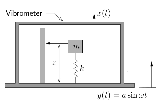
These instruments tend to be large and have soft springs so that their natural frequencies are small. As a result they are usually used in the range where  is large (
 ). In this range, we can see from Figure 5.13 that as ,
![\[\frac{\mathbb{Z}}{a} \longrightarrow 1\]](https://engcourses-uofa.ca/wp-content/ql-cache/quicklatex.com-938ed07eb41ec233a51024889422a1e5_l3.png "Rendered by QuickLaTeX.com")
so that the amplitude of the relative motion  between the mass and the base is the same as the amplitude
  of the actual motion of the base. In operation, the mass remains approximately stationary while the base moves with the supporting structure (whose vibrations are being measured).
These devices tend to have little damping, but as can be seen from Figure 5.13, even moderate
amounts of damping have only a small effect in this region.
Accelerometer
Accelerometers are widely used to measure acceleration levels. They tend to be small and stiff and as a result usually have very high natural frequencies. They are useful for measuring vibrations at frequencies that are much smaller than their own natural frequency ( ).
).
We can see from equation 5.34 that as approaches zero,
![\[\frac{\mathbb{Z}}{a} \longrightarrow \left(\ensuremath{\dfrac{\omega}{\ensuremath{p}}}\right)^2 \qquad\text{or}\qquad\mathbb{Z} \simeq \frac{1}{\ensuremath{p}^2} (a \omega^2)\]](https://engcourses-uofa.ca/wp-content/ql-cache/quicklatex.com-9f3ae8779d19e227d068beec4cbea69a_l3.png "Rendered by QuickLaTeX.com")
where  is the magnitude of the acceleration of the base. Therefore, in this region the amplitude of the relative motion is approximately proportional to the magnitude of the acceleration of the base.
To understand the response better, note that equation (5.34) could be rearranged as
![\[\mathbb{Z} = \frac{1}{\ensuremath{p}^2 } \bigl( a \omega^2 \bigr)\underbrace{\frac{1}{\ensuremath{\sqrt{\Bigl[1-\ensuremath{\bigl(\frac{\omega}{\ensuremath{p}}\bigr)}^2\Bigr]^2 + \Bigl[2 \zeta \ensuremath{\frac{\omega}{\ensuremath{p}}} \Bigr]^2}}}}_{\text{\small Factor } \approx 1}\]](https://engcourses-uofa.ca/wp-content/ql-cache/quicklatex.com-788420adf6e49c62abf7ba1e64580084_l3.png "Rendered by QuickLaTeX.com")
where  is a constant for the accelerometer that is usually determined by calibration.
As can be seen, the value of the factor
![\[\frac{1}{\ensuremath{\sqrt{\Bigl[1-\ensuremath{\bigl(\frac{\omega}{\ensuremath{p}}\bigr)}^2\Bigr]^2 + \Bigl[2 \zeta \ensuremath{\frac{\omega}{\ensuremath{p}}} \Bigr]^2}}}\]](https://engcourses-uofa.ca/wp-content/ql-cache/quicklatex.com-e4422c3c2883cf7214dbbc81f93f7338_l3.png "Rendered by QuickLaTeX.com")
approaches 1 as  but for
  this factor is different from one and this difference contributes to the error in the measurement.
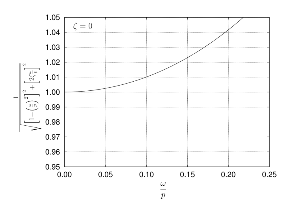
To see this effect, figure 5.14 illustrates this region of the response for an undamped accelerometer. For a frequency ratio  0.1, the value of the factor is approximately 1.01, which corresponds to approximately a 1
 error. At a frequency ratio 0.2, the value of the factor increases to approximately 1.04, which corresponds to a 4 error. Further increases in lead to rapidly increasing errors.
 ratios
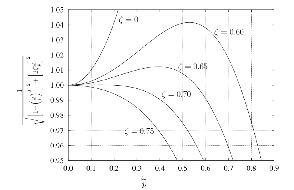 ratios
We can take advantage of damping to improve this behaviour. Figure 5.15 shows the effect of damping on the response. As shown in this figure, for damping ratios between about 0.65 and 0.7 this factor remains much closer to one over a wider range of frequency ratios. For example, with  0.7, the error introduced by assuming this factor to be unity is less than 1 over a frequency range of
  0.4, and is less than 0.01 for frequencies up to 20 of the natural frequency of the unit.
Many accelerometers, typically piezoelectric, have almost no damping so the usable frequency range is much smaller, up to about 10 of the natural frequency for a 1 error. Note however that these accelerometers tend to have quite large natural frequencies to begin with so the usable range is still quite appreciable.
Force Transmitted in Damped Base Excitation
During base excitation of a damped spring–mass system, the force transmitted between the support and the mass depends on the relative motion between the two and is transmitted through both the spring and the damper. Referring to Figure 5.11(b), the total force transmitted can be expressed as
(5.35) ![\[F_T = k \bigl( x-y \bigr) + c \bigl( \dot{x}-\dot{y} \bigr) \\\]](https://engcourses-uofa.ca/wp-content/ql-cache/quicklatex.com-741618ce8674f14dfc59bdcec800a102_l3.png "Rendered by QuickLaTeX.com")
or, in terms of the relative motion,
![\[F_T = k z + c \dot{z}\]](https://engcourses-uofa.ca/wp-content/ql-cache/quicklatex.com-96d0e9e8c948b8721421e7bd3b29787e_l3.png "Rendered by QuickLaTeX.com")
We could use either of these expressions since we have already found solutions for and  previously for this situation. However, it is much easier to proceed by comparing equations (5.35) and (5.23) to note that
![\[F_T= -m \ddot{x}\]](https://engcourses-uofa.ca/wp-content/ql-cache/quicklatex.com-5571e75ef11aaec6d2c814a2edf6089d_l3.png "Rendered by QuickLaTeX.com")
We have already shown (equation (5.28)) that the response of the mass is given by
![\[x(t) = \mathbb{X} \sin (\omega t - \phi)\qquad\text{where}\qquad\mathbb{X} = \frac{a \, \sqrt{1 + \bigl(2 \zeta \ensuremath{\frac{\omega}{\ensuremath{p}}} \bigr)^2}}{\ensuremath{\sqrt{\Bigl[1-\ensuremath{\bigl(\frac{\omega}{\ensuremath{p}}\bigr)}^2\Bigr]^2 + \Bigl[2 \zeta \ensuremath{\frac{\omega}{\ensuremath{p}}} \Bigr]^2}}}.\]](https://engcourses-uofa.ca/wp-content/ql-cache/quicklatex.com-51bc938ecc6e26b968fc00326b922c4a_l3.png "Rendered by QuickLaTeX.com")
so that the maximum acceleration is  . The maximum force transmitted is then
![\[\ensuremath{F_{\text{T}_\text{max}}} = m \Bigl[ \mathbb{X} \omega^2 \Bigr] = \left(\frac{k}{\ensuremath{p}^2}\right) \mathbb{X} \omega^2 =k \frac{\omega^2}{\ensuremath{p}^2} \frac{a \, \sqrt{1 + \bigl(2 \zeta \ensuremath{\frac{\omega}{\ensuremath{p}}} \bigr)^2}}{\ensuremath{\sqrt{\Bigl[1-\ensuremath{\bigl(\frac{\omega}{\ensuremath{p}}\bigr)}^2\Bigr]^2 + \Bigl[2 \zeta \ensuremath{\frac{\omega}{\ensuremath{p}}} \Bigr]^2}}},\]](https://engcourses-uofa.ca/wp-content/ql-cache/quicklatex.com-37ecd94aeade9bb764d730e40e18bb1d_l3.png "Rendered by QuickLaTeX.com")
which can be rearranged as
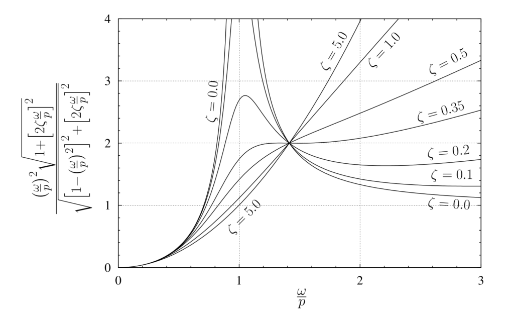
(5.36) ![\[\boxed{ \frac{\ensuremath{F_{\text{T}_\text{max}}}}{ka} = \frac{\ensuremath{\left(\dfrac{\omega}{\ensuremath{p}}}\right)^2 \sqrt{1 + \bigl(2 \zeta \ensuremath{\frac{\omega}{\ensuremath{p}}} \bigr)^2}}{\ensuremath{\sqrt{\Bigl[1-\ensuremath{\bigl(\frac{\omega}{\ensuremath{p}}\bigr)}^2\Bigr]^2 + \Bigl[2 \zeta \ensuremath{\frac{\omega}{\ensuremath{p}}} \Bigr]^2}}}}\]](https://engcourses-uofa.ca/wp-content/ql-cache/quicklatex.com-9799a1ea705bb36faea3e824f17e9987_l3.png "Rendered by QuickLaTeX.com")
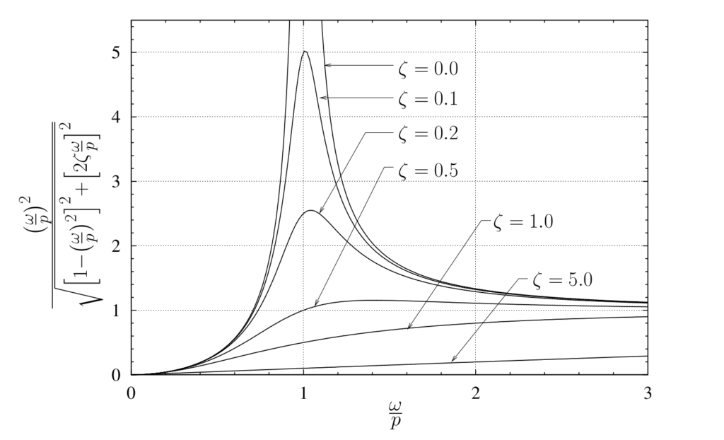
Equation (5.36) represents the transmissibility in the case of base excitation of a damped spring–mass system. As with the undamped situation discussed previously, the maximum disturbing force is again interpreted here to be  . Figure 5.16 represents this relationship.
why dont you consider the mass of the spring?
i just need to know that, if i consider the mass of the ‘moving spring’ also then the results[ x(t) ] would be changed??