
Equilibrium of Particles and Rigid Bodies: Conditions for two dimensional rigid-body equilibrium
In this section the conditions for equilibrium of a rigid body are presented. A rigid body, as previously defined, is an idealization of a body. A rigid body has a non-deformable shape meaning that loading or external forces does not change its shape. A rigid body consists of an infinite number of particles with fixed distances from each other. This implies that the equilibrium of a rigid body arises from the equilibrium of all its particles. Let’s consider the equilibrium of a rigid body consisting of four particles (Fig. 5.3a). The particles are represented by the circles and the distances between them are exaggerated. Assume that three of the particles are subject to external forces  .
.
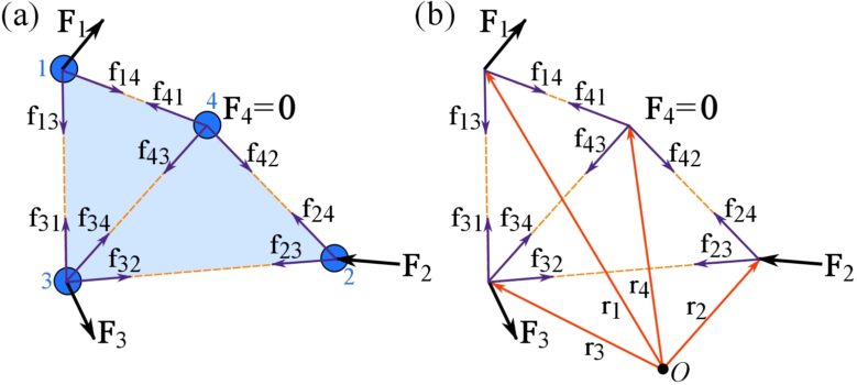
Since the body is rigid, the particles do not move relative to each other and therefore they maintain their initial distances. In addition to the external forces acting on the (three) particles, internal (intermolecular) forces exist among particles. These internal forces, schematically shown in Fig. 5.3b, are in the form of action-and-reaction forces (same magnitude but opposite directions) between each pair of the particles. The internal force acting on particle i by particle j is denoted as  .
.
Because each particle is in equilibrium, the equation of equilibrium for particles (Eq. 5.1) holds for each particle as,
![\[\begin{split}&\sum \bold F=\bold 0 \implies\\&\bold F_1 + \bold f_{13} + \bold f_{14} =\bold 0\\&\bold F_2 + \bold f_{24} + \bold f_{23} =\bold 0\\&\bold F_3 + \bold f_{31} + \bold f_{32} + \bold f_{34} =\bold 0\\&\bold f_{41} + \bold f_{42}+ \bold f_{43} =\bold 0\end{split}\]](https://engcourses-uofa.ca/wp-content/ql-cache/quicklatex.com-f43429aed1400e2e2956506e4ee0e894_l3.png "Rendered by QuickLaTeX.com")
As  , summing the above equations leads to,
![\[\sum \bold F =0 \implies \bold F_1+\bold F_2 + \bold F_3 = 0\]](https://engcourses-uofa.ca/wp-content/ql-cache/quicklatex.com-f4404507ab542275d6ec049da18b0eb6_l3.png "Rendered by QuickLaTeX.com")
This equation shows when the set of particles (or the body) is in equilibrium, the resultant (external) force on the rigid body (consisting of four particles) is zero. However, this only accounts for force (or translational) equilibrium. Unlike a particle, a rigid body has a size and couple forces can exist on two distant points of the body. Couple forces add up to zero, but they create couple moments that rotate the rigid body. Therefore, when a rigid body is in equilibrium, the sum of the couple moments should also be zero (the rotational equilibrium). This implies that the sum of moments of the forces at each particle about an arbitrary fixed point should be zero. Let  be an arbitrary point in the space , and
  be the quasi-moment-arms for the particles as shown in Fig. 5.3b, we have the following moment equilibrium equations for the particles.
![\[\begin{split}&\bold r_1\times (\bold F_1 + \bold f_{13} + \bold f_{14}) =\bold 0\\&\bold r_2\times (\bold F_2 + \bold f_{24} + \bold f_{23}) =\bold 0\\&\bold r_3\times(\bold F_3 + \bold f_{31} + \bold f_{32} + \bold f_{34}) =\bold 0\\&\bold r_4\times(\bold f_{41} + \bold f_{42}+ \bold f_{43}) =\bold 0\end{split}\]](https://engcourses-uofa.ca/wp-content/ql-cache/quicklatex.com-1883a4f2fa4b8d4a15d8e19015a1d311_l3.png "Rendered by QuickLaTeX.com")
Summing these equations with some mathematical manipulation leads to,
![\[\begin{split}&(\bold r_1\times\bold F_1) + (\bold r_2\times \bold F_2) + (\bold r_3\times \bold F_3)\\ &+(\bold r_1-\bold r_3)\times \bold f_{13}+(\bold r_1-\bold r_4)\times \bold f_{14}\\&+(\bold r_2-\bold r_3)\times \bold f_{23}+(\bold r_2-\bold r_4)\times \bold f_{24}\\&+(\bold r_3-\bold r_4)\times \bold f_{34}=\bold 0\end{split}\]](https://engcourses-uofa.ca/wp-content/ql-cache/quicklatex.com-e341eeac85733ea221029259b3d17371_l3.png "Rendered by QuickLaTeX.com")
The terms  , because the position (displacement) vector
  is parallel to . Therefore,
![\[(\bold r_1\times\bold F_1) + (\bold r_2\times \bold F_2) + (\bold r_3\times \bold F_3)=\sum \bold r\times F=(\bold M_R)_O=\bold 0\]](https://engcourses-uofa.ca/wp-content/ql-cache/quicklatex.com-9c73a6920178f3c8d3ab5a9e8fd20bc5_l3.png "Rendered by QuickLaTeX.com")
meaning that the sum of moments or the resultant moment of the external forces about equals zero.
In summary, if a rigid body is in equilibrium, the sum of the external forces and sum of the moments (including the couple moments) acting on the FBD of the rigid body are zero. It is also true reversely. If the resultant force,  and the resultant moment
  about any point are zero, the rigid body will be in equilibrium. These two equilibrium equations are formulated as,
(5.5) ![\[\begin{split}\bold F_R &= \sum \bold F = \bold 0\\(\bold M_R)_O&=\sum\bold M_O= \sum \bold r \times \bold F + \sum \bold M =\bold 0\end{split}\]](https://engcourses-uofa.ca/wp-content/ql-cache/quicklatex.com-6523b824bcc295fa3f32535a32b4c77b_l3.png "Rendered by QuickLaTeX.com")
In two dimensions, force systems are coplanar and moments about a point in the plane are perpendicular to the plane and the forces. The rigid body equations of equilibrium in a two-dimensional Cartesian coordinate system are,
![\[\begin{split}\sum \bold F_x &= 0\\\sum \bold F_y &= 0\\ \sum \bold M_O &= 0\end{split}\]](https://engcourses-uofa.ca/wp-content/ql-cache/quicklatex.com-7c6cbc92bb58b7fcc818b4448dd54d92_l3.png "Rendered by QuickLaTeX.com")
These equations are implemented using the scalar formulation (see Section 3.2) as,
(5.6) ![\[\begin{split}\sum F_x &= 0\\\sum F_y &= 0\\\circlearrowleft \sum M_O &= 0\end{split}\]](https://engcourses-uofa.ca/wp-content/ql-cache/quicklatex.com-a684c0243ed7e930829c51dc22c33008_l3.png "Rendered by QuickLaTeX.com")
where  indicates the direction of positive moments (counterclockwise). Recall that we use curved arrows to show the rotation tendency instead of the moment in two dimensional situations.
In two dimensions, there are three equations of equilibrium for a rigid body. Therefore, they can be solved for three unknowns. The unknowns can be a force (two unknown components) and a couple moment. To solve equilibrium problems in two dimensions, two steps must be followed:
1- Draw the FBD of the body. Isolate the body of interest from its surrounding. All supports and connections (joints with adjacent bodies) should be replaced with their reaction forces. Set a Cartesian coordinate system and express the forces by their rectangular components. Conveniently, the components of unknown forces are assumed in positive directions. The unknown couple moments are assumed positive, i.e. counterclockwise.
2- Write the equations of equilibrium and solve for the unknowns. Use the scalar formulation. Typically,
![\[\begin{split}\rightarrow \sum F_x &= 0\\\uparrow \sum F_y &= 0\\\circlearrowleft \sum M_O &= 0\end{split}\]](https://engcourses-uofa.ca/wp-content/ql-cache/quicklatex.com-ed8c1fa0a3040a4961873d120d63a2da_l3.png "Rendered by QuickLaTeX.com")
where  and
and  indicate the positive directions of the Cartesian axes.
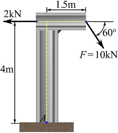
EXAMPLE 5.2.1
Determine the support reactions for the loaded structure shown in the figure.
SOLUTION
1- Draw the FBD of the structure.
Since the support of the structure is a fixed support, the support reactions are an unknown force and an unknown couple moment. If the force is expressed by its Cartesian components (in the positive Cartesian directions), and the couple moment is assumed positive, the FBD is,
Note that all the forces are decomposed into their Cartesian components.
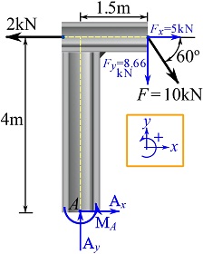
2- Write the equations of equilibrium and solve for the support reactions.
![\[\begin{split}\overset{+}{\rightarrow}\ \sum F_x&=0 \implies -2 + 5 + A_x=0\\+\uparrow\ \sum F_y&=0\implies -8.66+A_y=0\\\circlearrowleft \sum (M)_A &= 0\implies (2)(4)-(5)(4)-(8.66)(1.5)+M_A=0\end{split}\]](https://engcourses-uofa.ca/wp-content/ql-cache/quicklatex.com-e6a10d463c8525e8dfba02ee23ae6931_l3.png "Rendered by QuickLaTeX.com")
Solving the above equations results in,
![\[\begin{split}A_x&=-3\text{ kN}\implies A_x=3\text{ kN}\leftarrow\\A_y&=8.66\text{ kN}\\M_A&=25.0\text{ kN.m}\end{split}\]](https://engcourses-uofa.ca/wp-content/ql-cache/quicklatex.com-ca6f9e789800bab7d5eb87654ecfa8d2_l3.png "Rendered by QuickLaTeX.com")
Remark: don’t be confused with notations, : the couple moment at point
  .
. : the sum of moments (of forces and couple moments) about point .
EXAMPLE 5.2.2
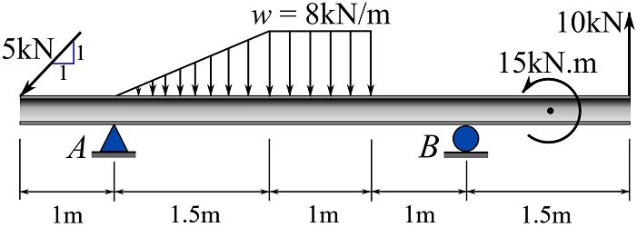
Considering the loaded beam shown, determine the support reactions.
SOLUTION
1- Draw the FBD. Simplify the distributed loads as concentrated loads (Section 3.5).
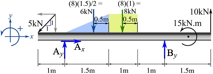
2- Write the equations of equilibrium and solve for the support reactions. Note the positive directions set by the Cartesian axes.
![\[\begin{split}\overset{+}{\rightarrow}\ \sum F_x&=0 \implies -5\frac{\sqrt{2}}{2} + A_x=0\\+\uparrow\ \sum F_y&=0\implies -5\frac{\sqrt{2}}{2} -6 - 8 + 10 +A_y + B_y=0\\\circlearrowleft \sum (M)_A &= 0\implies (5\frac{\sqrt{2}}{2})(1)-(6)(1)-(8)(2) + (B_y)(3.5) + 15 + (10)(5)=0\end{split}\]](https://engcourses-uofa.ca/wp-content/ql-cache/quicklatex.com-ef883239cccf39683f64d149cb2ef7af_l3.png "Rendered by QuickLaTeX.com")
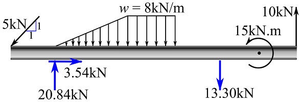
Solving the above equations (solve in the order of the first equation, the third one, and the second one), you get,
![\[\begin{split}A_x&=3.54\text{ kN}\rightarrow\\A_y&=20.84\text{ kN}\uparrow\\B_y&=-13.30\text{ kN}\implies B_y=13.3\text{ kN}\downarrow\\\end{split}\]](https://engcourses-uofa.ca/wp-content/ql-cache/quicklatex.com-e78001eae5bcf9ac2b2b27a33cef9ae3_l3.png "Rendered by QuickLaTeX.com")
The support reactions are shown as follows on the FBD,
The following interactive example shows how the support reactions change when the location of the load varies along the beam. Use the slider to move the load along the beam and note the support reactions; try to solve several cases yourself. In some cases you may observe that the support reaction of the roller becomes a pulling force on the beam. However, a roller model only supports pushing forces. In this case, assume that the support is a roller in a frictionless slot (see Table 4.1 Chapter 4).
Sometimes, the supports and/or connections, and loading conditions of a structural member can be used to determine the directions of forces acting on the member (it FBD). Two- and three-force members are such members.
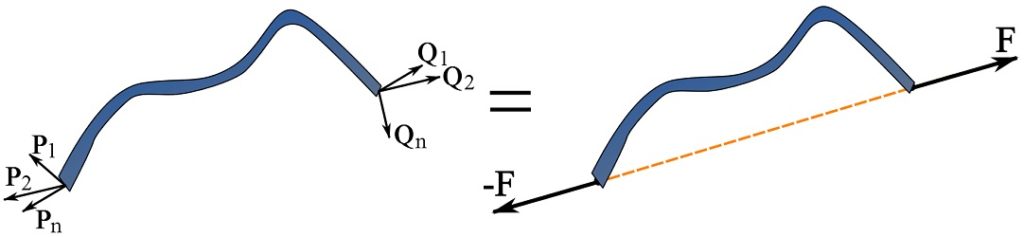
Two-force members. If a member is subjected to two resultant forces at two different locations and is in equilibrium, these two resultant forces must have the same line of action and be in opposite directions as shown in Fig. 5.4. Such a member is referred to as a two-force member. If a member acts as a two-force member, we can be certain that the two external resultant forces are equal in magnitude, collinear, and in opposite directions. Therefore, a two-force member appears with only one unknown which is the magnitude of the member force, in the equations of equilibrium. A common example of two-force members are truss members presented in Chapter 6.
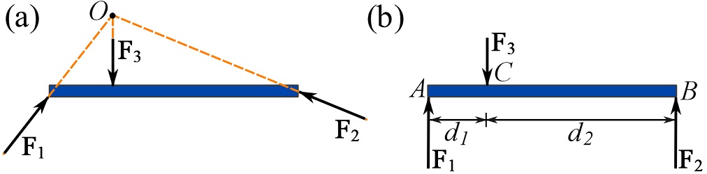
Three-force members. A three-force member is a member that is subjected to three resultant forces (on its FBD). The moment part of the equations of equilibrium is satisfied only if the lines of action of the three forces are either concurrent or parallel as shown in Fig. 5.5. This condition on the lines of action determines the directions of the forces and therefore reduces the number of unknowns.
Consider a three-force member with concurrent forces as shown in Fig 5.5a. The sum of moments about point where the forces are concurrent is zero. Therefore, the moment equilibrium  is satisfied.
For the case of parallel forces shown in Fig. 5.5b, the moment equilibrium about any points can be satisfied. For instance,
![\[\circlearrowleft \sum M_C=0\implies -(F_1)(d_1)+ (F_2)(d_2)=0\]](https://engcourses-uofa.ca/wp-content/ql-cache/quicklatex.com-43c529750e60d489e5899814ae293dcf_l3.png "Rendered by QuickLaTeX.com")
can be satisfied if  .
.
Project
This chapter contains a project in which you need to solve a problem related to a real engineering situation. To this end, please click here to view the project.
Videos
Force Equilibrium:
Static Equilibrium: