Engineering at Alberta Courses » Vector operations using the parallelogram rule and trigonometry

Vectors and their Operations: Vector operations using the parallelogram rule and trigonometry

The following are mathematical operations used for vectors in this course:

Multiplication (or division) by a scalar.
Vector addition (or subtraction).
Vector products (dot product and cross product).

The first two operations are the fundamental operations and are presented below. Vector products are special functions and presented in Sections 2.7 and 2.8.

Multiplication (and division) of a vector by a scalar

A vector can be multiplied by a scalar and the result is another vector. A vector $\bold A$ multiplied by a scalar $c$ will be equal the vector $\bold B$ . This operation is denoted as $\bold B = c\bold A$ . Division of a vector by a scalar $c\ne 0$ is the same as multiplication by $1/c$ . Multiplication of a vector by a scalar is implemented by the following rule:

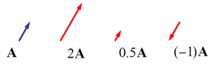
If the scalar is a positive number, scalar multiplication simply scales the magnitude (length) of a vector. If the scalar is negative, the operation also reverses the direction of the vector.

Remark: multiplying a vector by a scalar scales the vector’s magnitude: if $\bold B = c\bold A$ , then $\vert \bold B \vert=\vert c \bold A \vert =\vert c\vert \vert \bold A \vert$ in which $\vert c \vert$ is the absolute value of the scalar $c$ .

Remark: for any non zero scalar $a$ , if $c<0$ then $c\bold A$ scales and reverses (switches) the direction of $\bold A$ .

Remark: multiplication of any vector, $\bold A$ , by zero results in the zero vector: $0\bold A=\bold 0$ .

The following figure demonstrates different vectors as the results of multiplication of $\bold A$ by a scalar.

Fig. 2.4 Multiplication of a vector by a scalar.

Click on the following interactive tool demonstrates $\bold A$ multiplied by a scalar $\alpha$ to produce a new vector $\alpha \bold A$ . Move the slider to change the value of $\alpha$ and notice the effect on the resulting red vector. When does the vector $\alpha A$ reverse its direction?

Vector addition

The addition of vectors results in a new vector. For example, the addition of vectors $\bold A$ and $\bold B$ resulting in a vector $\bold C$ is denoted as $\bold A+\bold B=\bold C$ . There are two equivalent rules (laws) for vector addition: triangle rule, and parallelogram law.

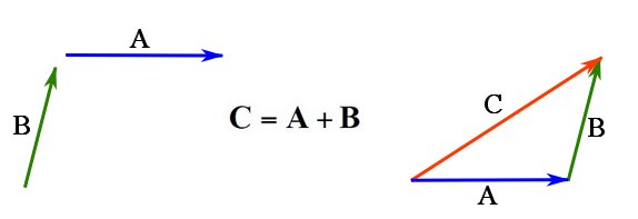
To calculate $\bold A+\bold B=\bold C$ using the triangle rule follow these steps:

Put $\bold A$ and $\bold B$ head to tail, and then,
Close the triangle with the vector $\bold C$ from the free tail to the free head of the vectors .

Fig. 2.5 demonstrates the triangle rule for vector addition.

Addition of two vectors by The triangle rule — Fig. 2.5 Graphical representation of the addition of vectors $\bold A$ and $\bold B$ using the triangle rule.

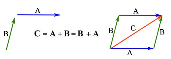
The vector addition is commutative meaning $\bold A+\bold B= \bold B+\bold A$ . This can be readily observed in the following figure:

Figure 2.6. Commutative property for the addition of vectors A and B. — Fig. 2.6 Commutative property for the addition of vectors $\bold A$ and $\bold B$ .

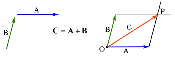
To add two vectors using the parallelogram law, follow these steps:

Bring the vectors to join at a point, say $O$ , by their tails.
From the head of each vector draw a line parallel to the other vector. These two lines intersect at a point $P$ and form two adjacent lines of a parallelogram.
Draw a vector from point $O$ to the point $P$ (the diagonal of the parallelogram). This vector is the resultant vector $\bold A + \bold B =\bold C$ .

Figure 2.7 demonstrates vector addition using the parallelogram law.

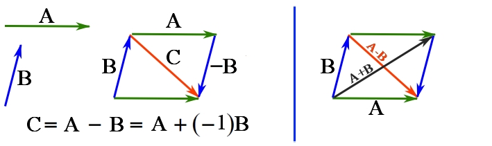
Vector subtraction. The difference between two vectors, or vector subtraction, follows the rules for vector addition. For two vectors $\bold A$ and $\bold B$ the operation $\bold A - \bold B$ can be written as $\bold A + (-1)\bold B =\bold A + (-\bold B)$ . An example is shown in Fig. 2.8.

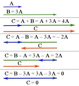
Remark: vector subtraction is not commutative because $\bold A - \bold B\ne \bold B - \bold A$ . In fact, $\bold A -\bold B = -(\bold B - \bold A)$ .

Addition (or subtraction) of parallel vectors. The addition (or subtraction) of parallel vectors is performed by bringing them head-to-tail and creating a longer or shorter vector. This means they are directly added (or subtracted) by their magnitudes.

Examples of vector addition (or subtraction) in the case of parallel vectors are demonstrated in Fig. 2.9.

Vector addition of parallel or colinear vectors. — Fig. 2.9 Vector addition of parallel vectors.

Addition of several vectors. If more than two vectors are to be added (or subtracted), they will be added successively. For example $\bold A + \bold B + \bold C=(\bold A + \bold B) + \bold C$ . An example is as demonstrated below:

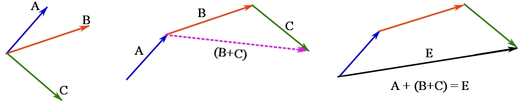Fig. 2.10 Successive addition of three vectors $\bold A$ , $\bold B$ and $\bold C$ using the triangle rule.

Experiment with the following interactive tool to investigate the parallelogram law for vector addition.

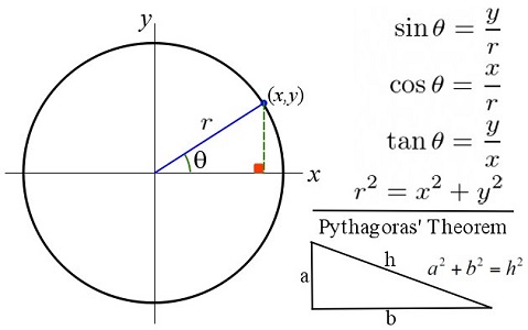
Trigonometry for vector operations

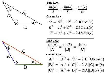
Trigonometric functions and laws are used to calculate the magnitude and direction of resultant vectors. The definition of the basic trigonometric functions are depicted in Fig. 2.11.

Fig. 2.11 Basic trigonometric functions.

Based on the trigonometric functions, the Sine and Cosine laws hold for any triangle or any three vectors forming a triangle. Fig. 2.12 demonstrates the Sine and Cosine laws hold for a triangle and for three vectors forming a triangle. In the case of vectors, the laws applies on the magnitudes of the vectors.

Fig. 2.12 Sine and Cosine Laws for a triangle (top) and for three vectors forming a triangle (bottom).

Remark: It should be understood that the magnitude of the resultant vector is not generally equal the addition of the magnitudes. In other words, $\vert \bold A + \bold B\vert \neq \vert \bold A \vert + \vert \bold B \vert$ . In fact, $\vert \bold A + \bold B\vert \le \vert \bold A \vert + \vert \bold B \vert$ always holds. This statement, called the triangle inequality, can be explored or proved by using the Cosine law.

The following interactive tool illustrates the trigonometric functions. Use the slider to vary the angle $\theta$ of the arrow and notice the corresponding changes in $\cos{\theta}$ and $\sin{\theta}$ . $\cos{\theta}$ is the signed length of the green dotted line and $\sin{\theta}$ is the signed length of the blue dotted line.

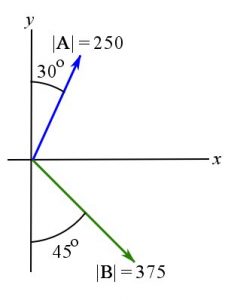
EXAMPLE 2.2.1

Determine the magnitude of the resultant vector $\bold C=\bold A+\bold B$ and its direction measured clockwise from the positive x-axis shown.

SOLUTION

Draw diagrams (parallelogram sides)
Show known information on the diagrams
Identify what to look for

Recall that Sine and Cosine Laws can be used to find angles and edge lengths, but more information is needed.

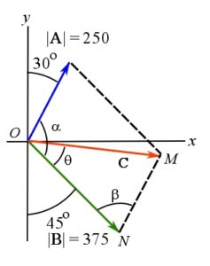
As a property of a parallelogram, $\angle$ $\alpha$ + $\angle$ $\beta$ = $180^{\circ}$

Therefore, $\angle \beta = 30^{\circ} + 45^{\circ} = 75^{\circ}$

For triangle $\triangle MNO$ , $OM$ (or $\bold C$ ) represents the resultant vector. From Cosine Law,

$\begin{split}OM^{2} &= ON^{2} + MN^{2} - 2(ON) (MN)( \cos{75^ {\circ}})\\&= 375^{2} + 250^{2} -(2)(375)(250) \cos{75^{\circ}}\\&\Rightarrow \ OM = 393.2 = |\bold C|\end{split}$

From Sine Law,

$\begin{split}\frac{\sin{\theta}}{NM}&= \frac{\sin{75^{\circ}}}{OM}\\\frac{\sin{\theta}}{250}&= \frac{\sin{75^{\circ}}}{(393.2)}\\\angle \theta&= 37.89^{\circ}\end{split}$

The angle of $\bold C$ with x axis is $7.11^\circ$ .

Videos

Vector Multiplication and Division by a Scalar:

Vector Addition using the Parallelogram Method: