Friction: Dry friction
Friction, generated at the interfaces of materials, is the force that opposes relative sliding motions of two solids, fluid layers, and material particles (molecular level). Types of friction are:
- Dry friction (Coulomb friction). Generated at the contact surfaces (interface) of two solids, dry friction is a force opposing the sliding of the solids against each other. This force is tangent to the surfaces in contact. Examples are force opposing sliding a box on a surface, frictional force at the contact area of a tire and road.
- Fluid friction. The force that resists motion of the sliding (shearing) layers of a fluid, or another object (a solid) moving within a fluid is referred to as fluid friction. Unlike dry friction with no fluid involved, fluid friction entails presence of fluid. Examples are the resisting force tangentially generated on the body of a swimmer in water, resisting force on the body of an airplane flying in the air. The friction between the air and smoke (particles) moving in the air is an example of fluid friction between layers of two fluids moving relative to each other.
- Internal Friction. This type of friction occurs at the molecular level within a material. An example is the appearance of internal friction that damps vibration of a string.
Mechanism of dry friction
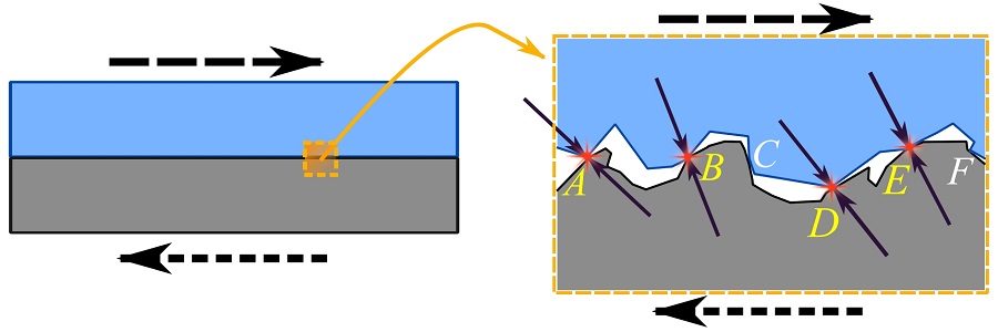
In reality, there is no perfectly smooth surface and all solid surfaces have a degree of roughness or irregularity in a microscopic level. To understand the mechanism giving rise to dry friction, it is necessary to consider the contact surfaces at a microscopic level.
Consider a cross section of two surfaces in contact with each other as shown in Fig 8.1. At a microscopic level, Fig. 8.1 shows how two solid contact surfaces might look in cross section when magnified.
As demonstrated in Fig. 8.1, when the upper surface slides or tends to slide to the right while the lower surface is stationary (or relatively moving to the left), the irregularities of the surfaces that come into contact exert forces on each other. The developed contact forces at the irregularities are indeed in the form of action-and-reactions according to Newton’s third law (Fig. 8.1). Also, the contact forces are normal to the local surfaces of the irregularities.
By the aforementioned mechanism of contact force development, the contact forces on the two sliding solid surfaces can be shown as Fig. 8.2a.
Now, let x be a direction tangent to the overall contact surface (i.e. sliding direction) and y a normal direction to the overall contact surface, i.e. sliding direction (Fig. 8.2b). Then, the contact forces at any of the local surfaces can be decomposed into the components  along the x direction and components
  being along the y direction as shown in Fig. 8.2b. The summations of the components in each of these two directions lead to the following resultant forces on each surface (Fig. 8.2c),
1)  is the friction force.
2)  is the normal force.
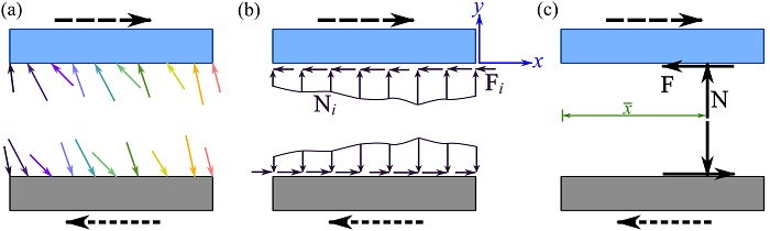
The location of the resultant normal force  to a surface is somewhere within the contact surface, e.g. denoted by
  in Fig. 8.2c. Calculating is not in the scope of this course and not going to be implemented.
Note that a frictional force developed on a surface is always in the direction opposing/preventing the sliding (or tendency of sliding). This can be observed in Fig. 8.2c.
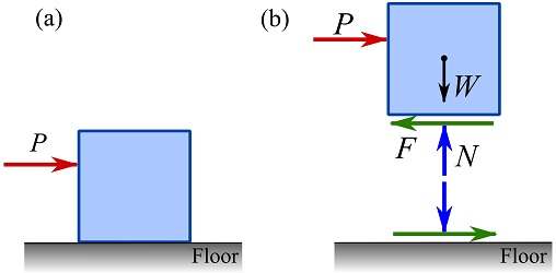
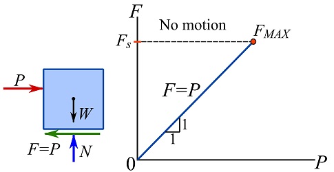
To investigate the characteristics of friction, consider a box initially resting on the floor (Fig. 8.3a) and a force  laterally exerted on the box as shown in Fig. 8.3a. The FBD of the box is sketched as in Fig. 8.3b. For simplicity, the system is assumed in two dimensions.
If  , the equilibrium in the horizontal direction indicates that
  i.e. no friction force acts on the box (Fig. 8.4). When
  gradually increases from zero, the box does not initially slide and the equilibrium of the box,
  indicates that
  . The relationship between and
  is sketched in Fig. 8.4. As continues to increase, increases as well. If the box does not tip over as increases, it will eventually start sliding over the floor. At the moment just before sliding, the maximum friction
  is achieved (Fig. 8.4). This situation is called impending slide or motion.
The maximum friction is called the (limiting) static friction,  , meaning the maximum friction that can be developed on contact surfaces just before the sliding. Physically,
  is directly proportional to the resultant normal force
  as the normal force affects the contact forces and interlocking the surface irregularities. If
  denotes the proportionality coefficient, the magnitude of static friction is,
(8.1) ![\[F_s=\mu_sN\]](https://engcourses-uofa.ca/wp-content/ql-cache/quicklatex.com-e6550a5917970d6117e381a93a63095b_l3.png "Rendered by QuickLaTeX.com")
The value of the coefficient of the static friction depends on the materials in contact, and is determined by experiments. Some examples are listed in table 8.1.
| Materials | |
| metal on ice | 0.03-0.05 |
| wood on wood | 0.25-0.50 |
| leather on metal | 0.60 |
| aluminum on aluminum | 1.35 |
| solids on rubber | 1-4 |
Increasing the lateral force on the box slightly beyond , will cause the box to slide (with increasing speed). Once sliding occurs, the magnitude of the frictional force drops to a smaller value denoted as  and called the kinetic friction (Fig 8.5). The kinetic friction is also proportional to the resultant normal force as,
(8.2) ![\[F_k=\mu_kN\]](https://engcourses-uofa.ca/wp-content/ql-cache/quicklatex.com-2b8633d1c3d34ca926c873da7b26518e_l3.png "Rendered by QuickLaTeX.com")
where  is called the coefficient of the kinetic friction. For a fixed value of normal force,
  , and therefore
  .
.
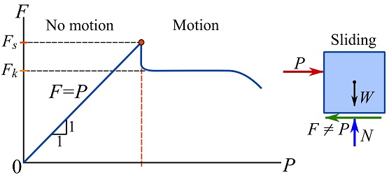
The physical reason explaining is that the sliding of the box causes the box to ride over irregularities. This lessens the interlocking of the irregularities of the two sliding surfaces.
Friction angles
At the onset of sliding (impending motion) when  , the angle of static friction is defined as,
Angle of static friction:  .
.
If  is the resultant of the frictional and normal forces, the geometric representation of
  , as demonstrated in Fig. 8.6, is the angle between
  and .
and .
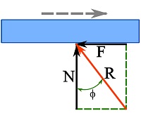
A friction angle with the same geometric representation can also be defined for kinetic friction:  .
.
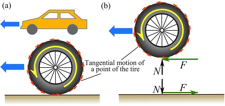
Friction on a rotating wheel
A rotating wheel in touch with the ground usually has a small contact area with the ground. The motions of the points of the wheel are tangent to the circumference of the wheel. When the wheel rotates, a frictional force exists at the contact area (point) and it prevents slipping of the wheel. As there is no slipping, the friction is static and  . Figure 8.7 shows an example of a wheel of a car rotating on the ground. The tires rotate counterclockwise (but no slip), and the static friction on the tire goes to the left. Therefore, the car can move to the left.