Engineering at Alberta Courses

Vectors and their Operations: Position vectors

Naturally, we can have a perception of a geometric point in space. A point in the space (three-dimensional or two-dimensional) can be imagined as an infinitely small dot. The space containing all the geometric points is called the geometric space. In a geometric space, geometric objects (or shapes) are born out of points. For examples, lines, circles, polylines, polygons, surfaces, cubes, etc. We simply refer to the geometric space as the space. The location of a point in the space can be quantitatively determined relative to other points. Thereby, all points can be located relative to one marked point. This point is called the origin of the space and denoted by $O$ . Generally, we form a Cartesian coordinate system in the space and define the origin of the space to be at the intersection of the three (or two) axes of the coordinate system. Therefore, any point in the space is identified by a coordinate triple $(x,y,z)$ in the three-dimensional space, or $(x,y)$ in the two-dimensional space. Obviously, the coordinates of the origin is $(0,0,0)$ . This approach was introduced by the French mathematician and philosopher René Descartes.

Another approach to locate (identify) a point in the space is by using a vector. Once a point in the space is marked as the origin, a vector (arrow) can be readily drawn (imagined) from the origin of the space, $O$ , to any point, $P$ , in the space. This vector is called the position vector of point $P$ relative to the origin. The position vector is generally denoted by $\bold r$ . 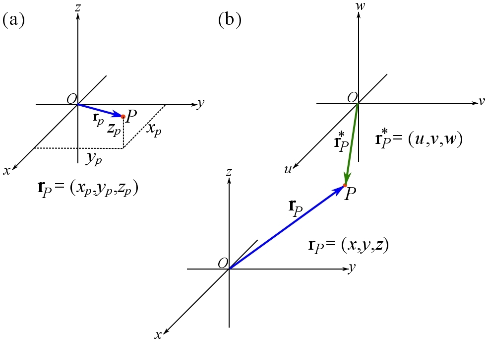To indicate a particular point located by a position vector, the notation $\bold r_{OP}$ or $\bold r_P$ is used. The former notation explicitly express the sense of the direction from the origin $O$ to the point $P$ , while the latter notation implicitly conveys the sense of the direction. A position vector simply points at a point in the space; its tail is at the origin of the space and its head is at any point to be located (Fig. 2.21a). Constructing a Cartesian coordinate system and the origin as well, the position vector can be represented in CVN as,

(2.10) $\bold r = x\bold i + y\bold j + z\bold k$

where $(x,y,z)$ are the coordinates of the point located by the position vector. Fig. 2.21a shows a position vector in a Cartesian coordinate system locating the points of a space.

A point, $P$ , in a the Cartesian coordinate system can be denoted by either of the following equivalent notations:

$\bold r_P=x_p\bold i + y_p\bold j + z_p\bold k$
$\bold r_p=(x_p,y_p,z_p)$
$P(x_p,y_p,z_p)$

Choosing a point as the origin of the space is arbitrary; however, a wise choice depending on the problem can simplify calculations. Fig. 2.21b shows a point in a space located (identified) by two different origins and position vectors. Note that the point is the same point but looked at from two different outlooks; therefore it has different coordinates and position vectors in the different coordinate systems.

Figure 20. Position vector and coordinate systems. — Fig. 2.21 Position vector and coordinate systems.

A position vector is a geometric object because it connects two geometric points in the space. This implies that the magnitude of a geometric vector $\vert \bold r\vert = \sqrt {x^2+y^2+z^2}$ has the dimension and units of length, and it measures the distance between two points.

Remark: unit of a position vector or its length has to be specified and written in the calculations. For example you can write $\bold r=\{a\bold i + b\bold j + c\bold k\}\ \text{m}$ where $(a,b,c)$ are the scalar components with the dimension of length and unit of meter, or for example $|\bold r|=7.0 \text{m}$ .

Using the coordinate direction angles $\alpha$ , $\beta$ , and $\gamma$ (measured from the positive $x$ , $y$ , and $z$ axes respectively), the following equations hold for a position vector in the Cartesian coordinate system.

(2.11) $\begin{split}\bold r &= x\bold i + y\bold j + z\bold k\quad\quad |\bold r|=\sqrt{x^2+y^2+z^2}\\x&=|\bold r|\cos \alpha\quad y=|\bold r|\cos \beta\quad z=|\bold r|\cos \gamma\quad \text{for } 0^\circ \le \alpha, \beta,\gamma \le 180^\circ\\ \bold u_r&=\frac{\bold r}{|\bold r|} \implies \bold u_r=(\cos\alpha)\bold i +(\cos\beta)\bold j+(\cos\gamma)\bold k \end{split}$

Remark: a unit vector $\bold u_r=\frac{\bold r}{|\bold r|}$ has no dimension. The unit vectors ( $\bold i, \bold j, \bold k$ ) of the coordinate system have no dimension as well.

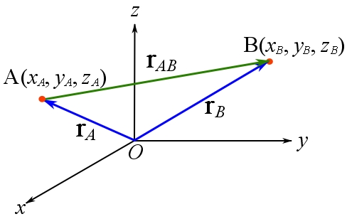
If a (geometric) vector connects two points, say $A$ and $B$ , in the space such that none of the points are designated as the origin, the vector is denoted by $\bold r_{AB}$ and called a displacement vector. The displacement vector in fact expresses the displacement of the position vector from point $A$ to point $B$ . To understand this concept, imagine two points $A$ and $B$ respectively located by the position vectors $\bold r_A$ and $\bold r_b$ in the coordinate system already having a defined origin $O$ and Cartesian coordinate axes (Fig. 2.22). The vector (arrow) from the point $A$ to the point $B$ is the displacement vector $\bold r_{AB}$ . By the rules of vector addition, we can write,

(2.12) $\bold r_A+\bold r_{AB}=\bold r_B \quad\text{or}\quad \bold r_{AB}=\bold r_B-\bold r_A$

By using CVN,

(2.13) $\bold r_{AB}= (x_B-x_A)\bold i+(y_B-y_A)\bold j+(z_B-z_A)\bold k$

Interpreting the above equations geometrically, we understand that if an object is displaced along the vector $\bold r_{AB}$ , its position is changed from the point $A$ , located by $\bold r_{A}$ , to the point $B$ located by $\bold r_B$ . The quantity $|\bold r_{AB}|$ is the length of the displacement.

Fig. 2.22. Position and displacement vectors. — Fig. 2.22 Position and displacement vectors.

One application of displacement vectors is to determine or set a direction for a line segment formed (line of action) between two points in the space, say $A$ and $B$ . This can be achieved through normalizing $\bold r_{AB}$ by writing $\bold u_{AB}=\frac{\bold r_{AB}}{|\bold r_{AB}|}$ . It should be noted that another possibility for setting a direction is normalizing $\bold r_{BA}$ which is in the opposite direction of $\bold r_{AB}$ .

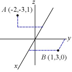
EXAMPLE 2.6.1

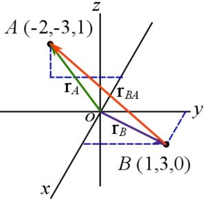
Find the position vector from point $B$ to point $A$ in CVN.

SOLUTION

Approach 1

$\begin{split}\bold r_{BA}&=\bold r_{OA}-\bold r_{OB}=\bold r_A-\bold r_B\\&=(-2\bold i-3\bold j+1\bold k)-(1\bold i+3\bold j+0\bold k)\\&=-3\bold i-6\bold j+\bold k\end{split}$

Approach 2

The scalar components can be directly found by subtracting the coordinates of the tail point from that of the tip point of the vector.

$\begin{split}\bold r_{BA}&=(x_A-x_B)\bold i+(y_A-y_B)\bold j+(z_A-z_B)\bold k\\&=(-2-1)\bold i+(-3-3)\bold j+(1-0)\bold k\\&=-3\bold i-6\bold j+\bold k\end{split}$

Note: since unit is not given, no unit is reported for the answers. The two vectors, $\bold r_{AB}$ and $\bold r_{BA}$ are in opposite directions, $\bold r_{AB}=-\bold r_{BA}=3\bold i+6\bold j-\bold k$ .

Context: Position Vectors

Forces carried by members depend on the angle of the member relative to applied forces (discussed further in Section 3.1.2 of this book).
In some systems and as part of the design process, engineers will know the physical start and end points of members. Based on these points, engineers can use position vectors to determine the magnitude (length) and direction (i.e. relative angles to the x, y, and z axes) of these members.
Position vectors are also a component of ‘moments’ (vectors that bend or twist members), which are introduced and formally defined in Section 3.2 of this book.

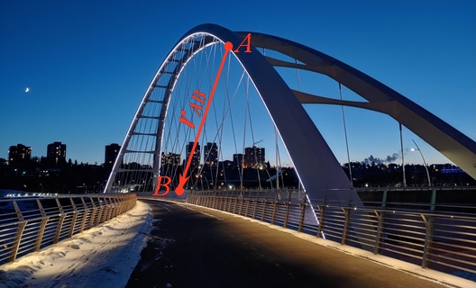
Applications: Why do we need position vectors?

The Walterdale Bridge in Edmonton (Fig. 2.23) opened in 2017 and spans around 200 m over the North Saskatchewan River. The bridge is comprised of two steel arches that support the roadway underneath using large cables. This bridge also has a large ‘shared use path’ (separate bridge that supports pedestrians, cyclists) on its east side.

Engineers need to know the length of each cable so that they can ensure that the cable manufacturer can build cables that are the correct length. Engineers also need to know the direction (i.e. relative angles) of each cable to determine how much force each cable carries under loading (a concept covered in Section 3.1.2 of this book). Using position vectors, both these unknowns can be determined.

Open Educational Resources

Vectors and their Operations: Position vectors

EXAMPLE 2.6.1

SOLUTION

Context: Position Vectors

Applications: Why do we need position vectors?

Video