Engineering at Alberta Courses » Analysis of trusses

Structural Analysis: Analysis of trusses

Trusses

One of the most common structures, especially for lightweight construction over long spans, is a truss. A truss consists of a number of long struts or bars (slender members) joined at their ends. The individual pieces are called members and the locations where they meet are called joints. Fig. 6.1 shows examples of trusses.

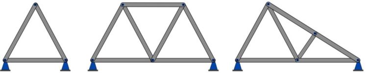
There are two main types of trusses, spatial and planar trusses (Fig. 6.1). A planar truss, being the topic of this chapter, is a truss with all its members lying in a plane. A common type of planar trusses is a simple truss. A simple truss consists of rigid triangular units in a way that the members of any unit do not cross members of other triangular units. Figure 6.2 shows examples of simple trusses.

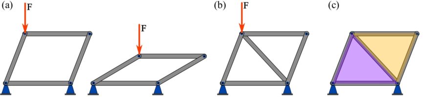
To better understand how a simple truss is created, consider the structure shown in Fig. 6.3a. This structure consists of bars joined at their ends using frictionless pins. If a force acts on the structure, the structure deforms and collapses (Fig. 63b). However, the structure becomes stable (rigid) if a diagonal member preventing the deformation is added as shown in Fig. 6.3b. This structure is now a simple truss; it consists of (non-crossing) triangle units (Fig. 6.3c). Each triangle is a rigid unit assuming that the bars are rigid.

Fig. 6.3 Creating a simple truss using rigid triangular units.

The main purpose of a structural analysis on a truss is to determine the internal forces of the members. The member forces are needed for designing the members and joints. To analyze a truss, two simplifying assumptions can be used. These assumptions, idealizing a real truss in practice, are as follows.

1- All loads act at the joints. It is assumed that loads being in the form of concentrated forces act at the joints of a truss (Fig. 6.4).

Fig. 6.4 Loads are applied at joints of a truss.

This assumption is almost true in practice; a physical truss performs optimally when the loads are applied at its joints. To achieve this, loads are transferred to the joints by beams or other structural members.

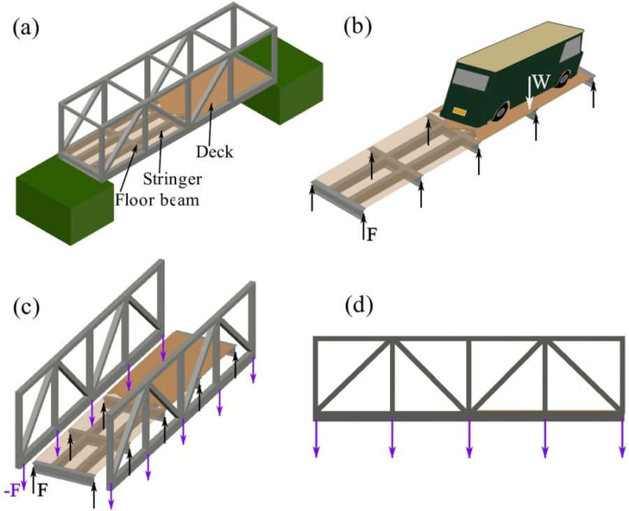
For example,consider a bridge with its deck connected to trusses through floor beams (Fig. 6.5a). The loads (weight of vehicles for example) on the deck are supported by the floor beams connected (at their ends) to the joints of the trusses. Figure 6.5b shows the FBD of the deck and beams of the bridge and the support reactions from the truss joints. Fig. 6.5c shows the action and reaction forces between the ends of the beams and the joints of the trusses. Finally, each truss is loaded as demonstrated in Fig. 6.5d.

Fig. 6.5 (a) A bridge with a deck supported by trusses, (b) FBD of the deck of the bridge, (c) load transfered from the deck and floor beams of the bridge to the joints of the trusses, (d) loads on the truss joints. Note that the (ground) support reactions of the truss are not shown.

The weight of the members of a truss are usually negligible in analysis as the weight of a member is much smaller than the member force. However, if the weights of a member are to be considered, a vertical force (in the direction of the gravity) being equal to half of the weight of the member is applied at each end of the member.

2- All joints act as frictionless pin connections.

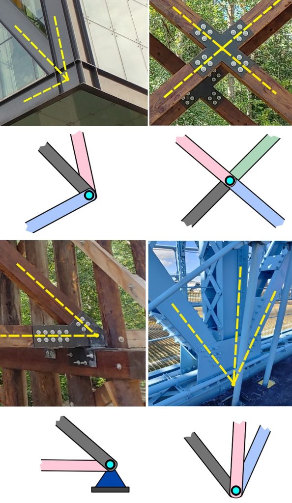
Joints are the locations in a truss where the ends of members concurrently meet. They include member-member joints, and member-support joints (Fig 6.6). It is ideal that the joints behave as frictionless pins (hinges); meaning that a joint does not restrain the rotation of the connected members. This assumption, used during analysis, is almost true in practice, as long as the members and therefore the lines of action of their forces, are concurrent at the joint. Consequently, the couple moment at the joint is small and negligible. For truss analysis, the point of concurrency (of the members’ axes) in a physical joint is considered as the location of the joint in the truss diagram. Figure 6.6 shows examples of joints and their truss diagrams.

Fig. 6.6 Physical trusses and their diagrams at joints.

The above assumptions result in a truss member acting as a two-force member. To prove this, a truss loaded with arbitrary loads is considered and one of its member ( $AB$ ) is arbitrarily chosen (Fig. 6.7a). Isolating the member $AB$ , we draw its FBD as shown in Fig. 6.7b.

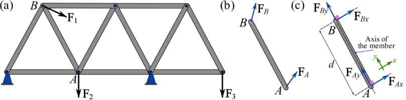Fig. 6.7 (a) A loaded truss (b) The FBD of the member $AB$ , (c) the components of the forces on the member.

Because each end of the member is a pin (hinge) connection, only a force (no moment) acts at each end. An end force can be decomposed along two directions being the member axis, $x$ , and an axis $y$ perpendicular to the member as shown in Fig.6.7c. The (planar) equations of equilibrium for the member are,

$\begin{split}\overset{+}{\rightarrow}\ \sum F_x&=0\implies F_{Ax}+F_{Bx}=0\\+\uparrow\ \sum F_y&=0\implies F_{Ay}+F_{By}=0\\\sum M_A&=0\implies F_{Bx}d=0\end{split}$

Solving the above equations determines the components of $\bold F_A$ and $\bold F_B$ as,

$\begin{split}F_{Bx}&= 0, F_{Bx}=0\\F_{Ay}&=-F_{By}\end{split}$

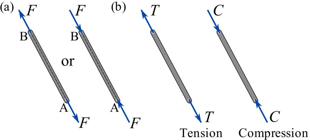
which indicates that $\bold F_A$ and $\bold F_B$ are along the axis of the member and $\bold F_A=-\bold F_B$ . Denoted by $\bold F$ , a member force can have either of the two cases shown in Fig 6.8a.

As shown in Fig. 6.8b, the force of a truss member is either a tensile (T) or a compressive (C) force acting at each end. The tensile force tends to elongate the member by pulling on it. The compressive force, on the other hand, tends to shorten the member by pushing on it.

Fig. 6.8 (a) possible types of forces of a truss member, (b) tension (T) and compression (C) forces of a truss member.

In truss analysis problems, member forces are unknown. There are two methods to solve for these forces, being the method of joints, and the method of sections. Both of these tactics will be expanded upon later in this chapter.

Context: Trusses

Trusses are a type of structural system. A structural system is a series of connected elements (also referred to as ‘members’) that carry loads (forces) to supports.
Relative to other types of structural members, truss members are easier to analyze as they are assumed to carry only axial forces (i.e. tension and compression).
Trusses have a high strength-to-weight ratio and are effective in a wide range of applications. However, connections between truss members, particularly those designed to resist heavy loads like those in bridges, can be very expensive to construct and maintain.
Many trusses can be idealized as planar trusses. We will focus on planar trusses in this book. There are some situations where engineers use space trusses (which need to be analyzed in three dimensions). The principles used to analyze planar trusses also apply to space trusses but the additional dimension makes calculations more complicated.

Applications: Where can I find trusses?

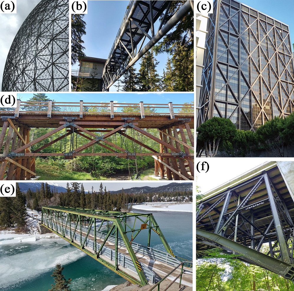
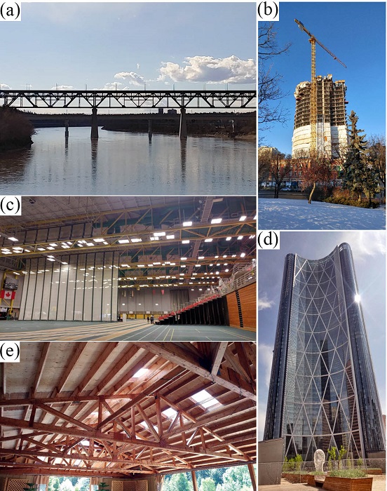
Truss bridges such as the High Level Bridge in Edmonton (Fig. 6.9a) are designed to carry heavy loads and span fairly long distances (longest span of 88 m in the case of the High Level Bridge). However, as mentioned earlier, construction and maintenance costs of the connections between members makes them less cost effective compared to other types of bridges (e.g. girder bridges) for modern applications. For this reason, most truss bridges you see are decades old.

Tower cranes (Fig. 6.9b) are made of trusses for various reasons but the primary reason is to make the crane as light as possible. This makes it easier to construct, deconstruct, and ship cranes from one site to the next on trucks.

Trusses are commonly used to support roofs, particularly those in buildings that require long spans (i.e. distances between supports) like those in athletic facilities (Fig. 6.9c) and airports. Unlike with bridges, roof trusses are protected against the elements so maintenance costs are lower. This makes trusses cost effective for long spans in modern low-rise buildings.

Truss members are also commonly used in steel buildings to resist lateral loads (sideways forces that come from wind and earthquakes). A prominent example of trusses being used as a lateral load resisting system is The Bow skyscraper in Calgary (Fig. 6.9d) which was the tallest building in western Canada when it was completed in 2012. To limit how much The Bow sways when the wind is blowing (which would make occupants uncomfortable), large trusses were added on the building which makes for a dramatic structural (as well as architectural) feature. Most buildings are more modest (e.g. DICE at the University of Alberta) with their lateral load resisting systems but also use truss members to prevent them from swaying excessively.

Trusses do not need to be made of steel. Though wood is much weaker than steel it is lightweight, cheap, and easy to work with (i.e. it can be assembled with hand tools). Wooden trusses similar to the one shown in Figure 6.9e are commonly used to support roofs in houses. The triangular shape of these trusses also makes it easier to construct sloped roofs.

Fig. 6.9 Trusses used in various applications (a) High Level Bridge, Edmonton (opened in 1913) (b) tower crane used for the construction of a high rise condo tower in Edmonton (c) Universiade Pavilion (commonly referred to as the ‘Butterdome’ because it looks like a stick of butter) fieldhouse at the University of Alberta (opened in 1983), (d) The Bow skyscraper, Calgary, (opened in 2012), and (e) Wood roof truss used in a low-rise structure (photos by D. Tomlinson).

The method of joints

If a truss is in equilibrium, its joints are also in equilibrium. By virtue of this, the equilibrium equations of a joint can be used to determine the member forces. To draw the FBD of a joint, it should be noted that the member forces are exerted by the joints. In other words, the members exert forces to the joint and the joint reacts with forces of the same magnitude and opposite directions (action and reaction). Figure 6.10 shows the FBD of a joint of a truss. To isolate a joint, we can either imaginarily cut around the joint as in Fig 6.10a, or disassemble the members from the connecting (pin) joint as shown in Fig. 6.10b. Both methods lead to the same result: the FBD of the joint. Since the members can be in tension or compression, we don’t know the sense of the member forces before analysis. Therefore, in the FBD, we can assume the senses of the member forces.

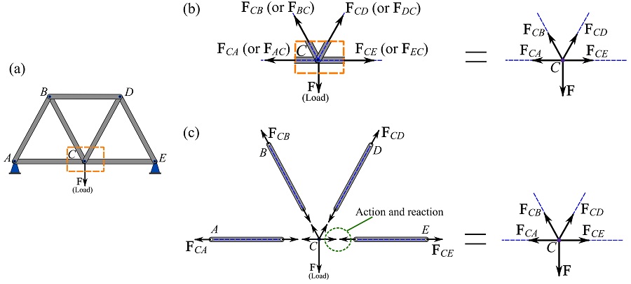
Each FBD is drawn from the perspective of the joint as an isolated body (particle); thus, all forces (even internal member forces) are external forces to the joints. The force of a member is labeled by referring to the labels of the ends (joints) of the member (e.g. $\bold F_{CA}$ or $\bold F_{AC}$ as in Fig. 10). The same label is used in the FBD of the joints.

As already shown in Fig 6.6b and Fig 6.10, a joint is considered to be a point at which member forces are concurrent. Therefore, in truss analysis, a joint can be modeled as a particle and the particle equilibrium equations (the scalar formulation) from Section 5.1 can be applied here,

$\begin{split}\sum F_x &= 0\\\sum F_y &= 0\end{split}$

Since there are two equations of equilibrium at each joint, two unknown member forces at most can be determined per joint. The line of actions of the forces at each joint are already known (they are along the members as explained in the previous section). Therefore, the equations are used to determine the magnitudes and sense of direction (i.e. tension or compression) . The method of joints is illustrated by the following example.

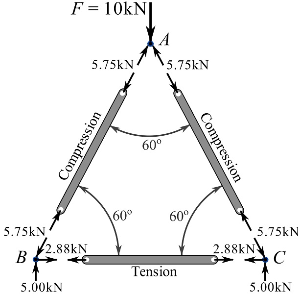
Consider the simple truss shown in Fig. 6.11a. We consider joint $A$ to determine the forces of the members $AB$ and $AC$ through the following procedure.

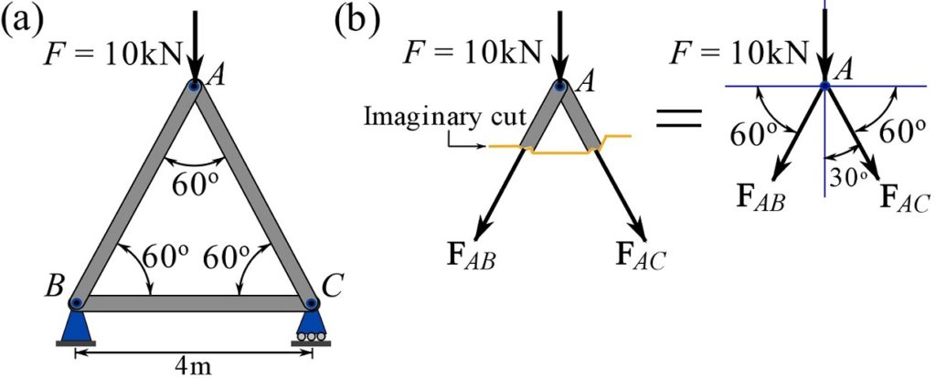
Fig 6.11 (a) A loaded truss, (b) the FBD of joint A.

1- Draw the FBD of joint A. Isolating joint A from its surroundings (Fig. 6.11b), we consider the external load and the member forces at the joint. The member forces are assumed as tensile forces (Fig 6.11b) and therefore pointing away from the joint. Since the number of unknown member forces is two, they can be solved for using the equations of equilibrium of joint A.

2- Write the equations of equilibrium for joint A. Using the components of the forces and following the scalar formulation (Section 5.1) we can write,

$\begin{split}\overset{+}{\rightarrow}\ &\sum F_x=0 \implies F_{AB}\cos 60^\circ - F_{AC}\cos 60^\circ = 0\\+\uparrow\ &\sum F_y=0\implies -10 - F_{AB}\sin 60^\circ-F_{AC}\sin60^\circ=0\\\end{split}$

where $F_{AB}$ and $F_{AC}$ are the magnitudes of the components and the signs in front them are determined based the directions of the components in the FBD.

3- Solve for the magnitudes of the unknown member forces. The equations of equilibrium can now be solved for the force magnitudes $F_{AB}$ and $F_{AC}$ .

$\begin{cases}0.50F_{AB}- 0.50F_{AC}=0\\0.87F_{AB}+0.87F_{AC}=-10\\\end{cases}\implies F_{AB}=-5.75\text{ kN},\quad F_{AC}=-5.75\text{ kN}$

4- Identify the true sense of directions (tension or compression). Any negative solution indicates that the sense of direction of the force was incorrectly assumed. As we initially assumed a tensile force for a member, any negative value (of a magnitude) implies that the force should be a compressive force and the true direction in the FBD should be the opposite. In this example, $F_{AB}$ and $F_{AC}$ are negative, therefore, they are compressive forces and we write,

$\therefore F_{AB}=5.75\text{ kN (C)},\quad F_{AC}=5.75\text{ kN (C)}$

where “(C)” denotes compression or compressive.

To avoid potential confusion, we need to be consistent in assuming the direction of unknown forces, such as all members in tension. In this way, we can identify the true senses quickly, negative values mean compression, positive means tension.

The same procedure can be followed to find the force in member $BC$ . This member connects joints $B$ and $C$ . The FBDs of joint $B$ and $C$ are shown in Fig. 6.12.

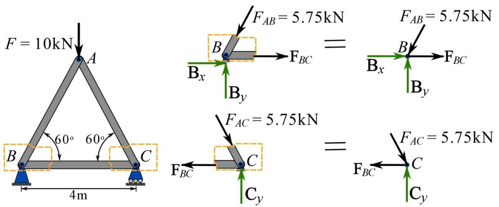
Joint $B$ has two unknown support reactions in addition to the unknown member force $\bold F_{BC}$ , therefore the two equations of equilibrium cannot be solved for three unknowns. However, there are two unknowns, a support reaction and the unknown member force $\bold F_{BC}$ at joint $C$ . Choosing node $C$ , we write,

$\begin{split}\overset{+}{\rightarrow}\ &\sum F_x=0 \implies -F_{BC} + 5.75\cos 60^\circ = 0\implies F_{BC}= 2.88 \text{ kN}\\+\uparrow\ &\sum F_y=0\implies C_y - 5.75\sin 60^\circ\implies C_y= 5.00 \text{ kN}\\\end{split}$

Therefore,

$F_{BC}= 2.88\text{ kN (T)}$

where “(T)” denotes tension or tensile.

Figure 6.13 demonstrates all the determined member and joint forces on their FBDs.

As it can be observed, the support reaction $C_y$ is also determined. We may choose not to solve for the support reactions if not needed. In this problem though, the support reactions can be obtained by writing the equations of equilibrium for the whole truss (try it yourself).

The method of joints may be utilized to completely determine the member forces of a truss. The following hints are useful when tackling a truss analysis problem using the method of joints.

Consider the FBD of the whole truss and determine support reactions. Support reactions are external loads to the corresponding joints of the FBD of the truss.
Start solving the unknown member forces at joints with one or at most two unknown forces.
Finding the zero-force members simplifies the problem. Zero-force members are explained below.

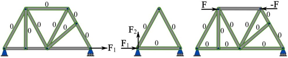
Zero-force members. Zero-force members are the members that do not carry any member forces. In some cases, due to the external loading situations and/or support designs, a member can behave as a zero-force member. In the first two cases demonstrated below, the zero force members can be easily identified by observation.

1- Two non-collinear members forming a joint are zero-force members if the joint is not externally loaded or not connected to a support. Figure 6.14a shows a general case of this type of zero-force members, i.e. members $AB$ and $AC$ .

Fig. 6.14 (a) Zero-force members AB and AC, (b) The FBD’s of joint A.

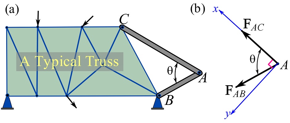
To prove that members $AB$ and $AC$ are zero-force members, the FBD of joint $A$ is considered as shown in Fig. 6.14b. Setting a Cartesian coordinate system with the x axis being in the direction of $\bold F_AC$ and therefore the y axis perpendicular to the x axis as shown, we can write the equilibrium equations as,

$\begin{split}+\nwarrow \sum F_x&=0\implies F_{AC} + F_{AB}\cos\theta = 0\\+\swarrow \sum F_y &=0\implies F_{AB}\sin \theta = 0\end{split}$

which implies, $F_{AB}=0$ and $F_{AC}=0$

Figure 6.15 shows examples of zero-force members.

Fig. 6.15 The members AB, BC, DE, and EF are zero-force members under the loading conditions shown.

2- A member connected to two collinear members at the same joint is a zero-force member if the joint is not externally loaded or has support reactions. َMember $AB$ shown in Fig 6.16a is a general case of this kind of zero-force member.

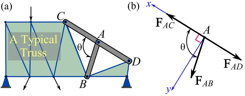
Fig. 6.16 (a) Zero-force member AB, (b) The FBD’s of joint A.

To prove that member $AB$ is a zero-force member, the FBD of joint $A$ is considered as shown in Fig. 6.16b. Setting a Cartesian coordinate system with the x axis being along the line of action of the collinear member forces $\bold F_AC$ and $F_AD$ and the y axis perpendicular to the x axis (Fig. 6.16b), we can write the equilibrium equations as,

$\begin{split}+\swarrow \sum F_y &=0\implies F_{AB}\sin \theta = 0\end{split}$

which implies $F_{AB}=0$ .

Figure 6.17 shows examples of zero-force members due to being connected to collinear members as explained.

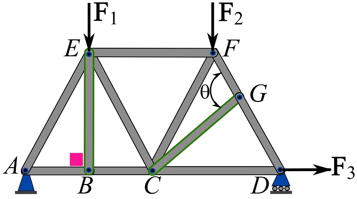
Fig. 6.17 The members BE and CG are zero-force members under the loading conditions shown.

3- There are other situations leading to zero-force members; some examples are shown in Fig. 6.18.

Fig. 6.18 Examples of zero-force members.

Remark: a member can be a zero-force member in some loading situations and be a non-zero force member in other loading situations. For example, if a force is added at joint B in Fig. 6.14, then members $BC$ and $BA$ are no more zero-force members. Therefore, for a member being a zero-force member depends on the loading of the truss. Although a zero-force member has no force (under a particular loading of a truss), it serves the stability, and rigidity of the truss.

The method of sections

In the method of joints, we need to start the analysis at a joint with a maximum of two unknown forces. Then, going from joint by joint until the member forces of interest are obtained. This procedure may be cumbersome if the member of interest is far from the joint we start with. As an alternative, the method of sections may give us a faster solution.

The method of sections is based on the fact that if a planar truss is in equilibrium, any section of the truss is also in equilibrium. Therefore, any section separated by an imaginary cut from the truss is a rigid body in equilibrium and the following equations of equilibrium hold for the FBD of the section.

$\begin{split}\sum F_x &= 0\\\sum F_y &= 0\\\sum M_O &= 0\end{split}$

where $O$ is a point in the plane of the truss (on the truss or not). The three equations of equilibrium can be solved for at most three unknowns. The unknowns in an analysis of a truss can be the member forces or/and the support reactions. This method is illustrated through the following example.

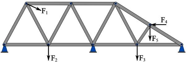
Consider the truss shown in Fig. 6.19. The forces in the members $EG$ , $EF$ , and $DF$ are to be determined. We take the following steps to determine the forces.

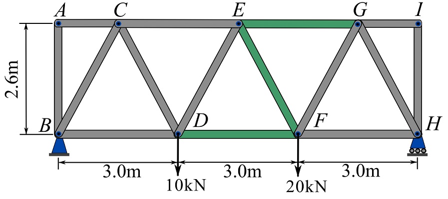
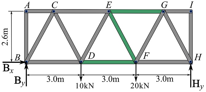
1- Determine the support reactions. For this problem, we need to determine the support reactions and use them for other equilibrium equations later. In some cases, we may not need to know the support reactions. The support reactions can be determined by solving the equations of equilibrium of the truss as one rigid body. Considering the FBD of the truss (Fig. 6.20), we write,

$\begin{split}\overset{+}{\rightarrow}\ \sum F_x &= 0 \implies B_x=0\\+\uparrow\ \sum F_y &= 0 \implies B_y + H_y -10-20 = 0\\\circlearrowleft{+} \sum M_B &=0\implies\ (H_y)(9)-(20)(6)-(10)(3)=0\end{split}$

which leads to,

$B_x=0,\quad B_y=13.3 \text{kN} \uparrow ,\quad H_y= 16.7 \text{kN} \uparrow$

2- Select Section(s) of the truss. An imaginary cut is made through the three members in the question and separate the truss into two sections as Fig. 6.21a.

3- Draw the FBD of the sections. The FBDs of the two sections are drawn as shown in Fig 6.21b and 6.21c. Note that the member forces are now exposed as external forces.

4- Choose a section. Generally, a section with a lesser number of unknowns should be chosen. In this problem, both segments have three unknowns (the member forces). Therefore, either segment can be chosen. We choose section 1 for further illustration. As we can observe, the support reactions would add to the unknowns if they were not already determined.

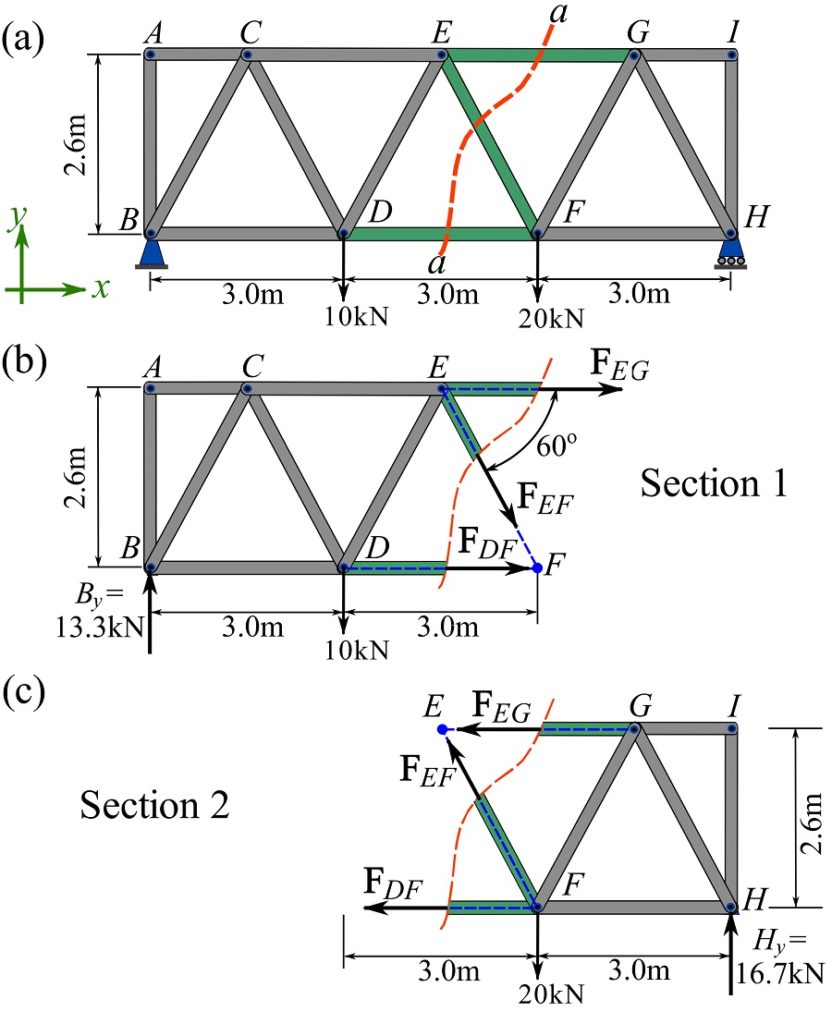
Fig. 6.21 Sections (and their FBDs) produced.

5- Write the equations of equilibrium and solve for the unknowns. By investigating the section, we find out that writing the moment equilibrium about point $F$ will lead us to $F_{EG}$ . Thereby,

$\begin{split}\circlearrowleft{+} \sum M_F &=0\implies\ -(13.3)(6.0) + (10)(3.0) - (F_{EG})(2.6)=0\\\implies F_{EG} &= -19.2\\\therefore F_{EG}&= 19.2\text{ kN (C)}\end{split}$

The equilibrium equation in the $y$ direction then leads to $F_{EF}$ as,

$\begin{split}+\uparrow\ \sum F_y &= 0 \implies 13.3 -10 - F_{EF}\sin 60^\circ = 0\\\implies F_{EF}&= 3.8\\\therefore F_{EF}&= 3.8\text{ kN (T)}\end{split}$

And eventually, the equilibrium equation in the x directions determines $F_{DF}$ as,

$\begin{split}\overset{+}{\rightarrow}\ \sum F_x &= 0 \implies F_{EG} + F_{EF}\cos 60^\circ + F_{DF}= 0\implies -19.2 + 3.8\cos 60^\circ + F_{DF} = 0\\\implies F_{DF} &= 17.3\\\therefore F_{DF}&= 17.3\text{ kN (T)}\end{split}$

The following interactive tool solves the member forces and support reactions of a truss under particular loads. Change the magnitude of the load (input box), sense of direction of a load (check box), and the location of a load (using a slider), and press SOLVE to observe the results. To remove a load, insert 0 as its magnitude (the input box should have a value).

Project

This chapter contains a project in which you need to solve a problem related to a real engineering situation. To this end, please click here to view the project.

Videos

Introduction to Trusses:

Truss Internal Forces and Stability:

Zero-Force Members:

Truss Analysis (Method of Joints):

Truss Analysis (Method of Sections):